LOCALLY WEIGHTED REGRESSION

• The phrase "locally weighted regression" is called local because the function is approximated based only on data near the query point, weighted because the contribution of each training example is weighted by its distance from the query point, and regression because this is the term used widely in the statistical learning community for the problem of approximating real-valued functions.
• Given a new query instance xq, the general approach in locally weighted regression is to construct an approximation 𝑓̂ that fits the training examples in the neighborhood surrounding xq. This approximation is then used to calculate the value 𝑓̂(xq), which is output as the estimated target value for the query instance. 

Locally Weighted Linear Regression

• Consider locally weighted regression in which the target function f is approximated near xq using a linear function of the form

Where, ai(x) denotes the value of the i^th attribute of the instance x

• Derived methods are used to choose weights that minimize the squared error summed over the set D of training examples using gradient descent

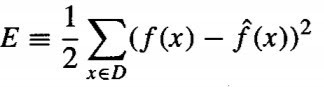
Which led us to the gradient descent training rule

Where, η is a constant learning rate

• Need to modify this procedure to derive a local approximation rather than a global one. The simple way is to redefine the error criterion E to emphasize fitting the local training examples. Three possible criteria are given below.

1. Minimize the squared error over just the k nearest neighbors:

2. Minimize the squared error over the entire set D of training examples, while weighting the error of each training example by some decreasing function K of its distance from xq :

3. Combine 1 and 2:

If we choose criterion three and re-derive the gradient descent rule, we obtain the following training rule

The differences between this new rule and the rule given by Equation (3) are that the contribution of instance x to the weight update is now multiplied by the distance penalty K(d(xq, x)), and that the error is summed over only the k nearest training examples.