Quick sort

The Quicksort Algorithm

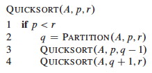
To sort any subarray A[p .. r], p < r:

Divide: Partition A[p .. r] into two (possibly empty) subarrays

• A[p .. q-1], where every element is ≤ A[q]
• A[q + 1 .. r], where A[q] ≤ every element Conquer: Sort the two subarrays by recursive calls Combine: No work is needed to combine: all subarrays (including the entire array) are sorted as soon as recursion ends.

An array is sorted with a call to QUICKSORT(A, 1, A.length):

The work is done in the PARTITION procedure. A[r] will be the pivot. (Note that the end element of the array is taken as the pivot. Given random data, the choice of the position of the pivot is arbitrary; working with an end element simplifies the code):

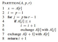
PARTITION maintains four regions.

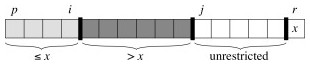
Three of these are described by the following loop invariants, and the fourth (A[j .. r-1]) consists of elements that not yet been examined:

Loop Invariant:

All entries in A[p .. i] are ≤ pivot.

All entries in A[i+1 .. j-1] are > pivot.

A[r] = pivot.

Example Trace

It is worth taking some time to trace through and explain each step of this example of the PARTITION procedure, paying particular attention to the movement of the dark lines representing partition boundaries.

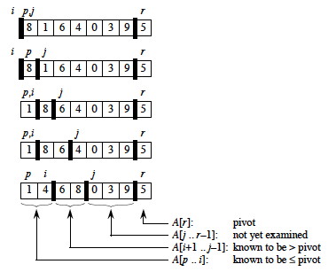
Continuing …

Correctness

Here use the loop invariant to show correctness:

1. All entries in A[p .. i] are ≤ pivot.
2. All entries in A[i+1 .. j −1] are > pivot.
3. A[r] = pivot.

Initialization: Before the loop starts, x is assigned the pivot A[r] (satisfying condition 3), and the subarrays a[p .. i] and A[i+1 .. j−1] are empty (trivially satisfying conditions 1 and 2). Maintenance: While the loop is running,

• if A[j] ≤ pivot, then i is incremented, A[j] and A[i] are swapped, and j is incremented. Because of the swap, A[i] ≤ x for condition 1. The item swapped into A[j-1] > x by the loop invariant, for condition 2.
• If A[j] > pivot, then j is incremented, sustaining condition 2 (the others are unchanged), as the element added was larger Termination: The loop terminates when j=r, so all elements in A are partitioned into one of three cases: A[p .. i] ≤ pivot, A[i+1 .. r-1] > pivot, and A[r] = pivot. The last two lines fix the placement of A[r] by moving it between the two subarrays.

---

Informal Analysis

The formal analysis will be done on a randomized version of Quicksort. This informal analysis helps to motivate that randomization.

First, PARTITION is Θ(n): We can easily see that its only component that grows with n is the for loop that iterates proportional to the number of elements in the subarray).

The runtime depends on the partitioning of the subarrays:

Worst Case

The worst case occurs when the subarrays are completely unbalanced, i.e., there are 0 elements in one subarray and n-1 elements in the other subarray (the single pivot is not processed in recursive calls). This gives a familiar recurrence (compare to that for insertion sort):

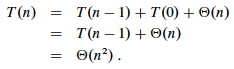
One example of data that leads to this behavior is when the data is already sorted: the pivot is always the maximum element, so we get partitions of size n−1 and 0 each time. Thus, quicksort is O(_n_2) on sorted data. Insertion sort actually does better on a sorted array! (O(n))

Best Case

The best case occurs when the subarrays are completely balanced (the pivot is the median value): subarrays have about n/2 elements. The reucurrence is also familiar (compare to that for merge sort):

Effect of Unbalanced Partitioning

It turns out that expected behavior is closer to the best case than the worst case. Two examples suggest why expected case won’t be that bad.

Example: 1-to-9 split

Suppose each call splits the data into 1/10 and 9/10. This is highly unbalanced: won’t it result in horrible performance?

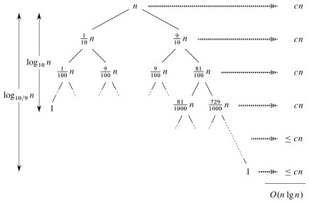
We have log10_n_ full levels and log10/9_n_ levels that are nonempty.

As long as it’s constant, the base of the log does not affect asymptotic results. Any split of constant proportionality will yield a recursion tree of depth Θ(lg n). In particular (using ≈ to indicate truncation of low order digits),

log10/9_n_ = (log2_n_) / (log210/9) by formula 3.15

≈ (log2_n_) / 0.152

= 1/0.152 (log2_n_)

≈ 6.5788 (log2_n_)

= Θ(lg n), where c = 6.5788.

So the recurrence and its solution is:

A general lesson that might be taken from this: sometimes, even very unbalanced divide and conquer can be useful.

Example: extreme cases cancel out

With random data there will usually be a mix of good and bad splits throughout the recursion tree.

A mixture of worst case and best case splits is asymptotically the same as best case:

Both these trees have the same two leaves. The extra level on the left hand side only increases the height by a factor of 2, and this constant disappears in the Θ analysis.

Both result in O(n lg n), though with a larger constant for the left.at they exist.