Curve Clipping and Text clipping

Text Clipping

Various techniques are used to provide text clipping in a computer graphics. It depends on the methods used to generate characters and the requirements of a particular application. There are three methods for text clipping which are listed below −

• All or none string clipping
• All or none character clipping
• Text clipping

The following figure shows all or none string clipping –

In all or none string clipping method, either we keep the entire string or we reject entire string based on the clipping window. As shown in the above figure, STRING2 is entirely inside the clipping window so we keep it and STRING1 being only partially inside the window, we reject.

The following figure shows all or none character clipping –

This clipping method is based on characters rather than entire string. In this method if the string is entirely inside the clipping window, then we keep it. If it is partially outside the window, then −

• You reject only the portion of the string being outside
• If the character is on the boundary of the clipping window, then we discard that entire character and keep the rest string.

The following figure shows text clipping –

This clipping method is based on characters rather than the entire string. In this method if the string is entirely inside the clipping window, then we keep it. If it is partially outside the window, then

• You reject only the portion of string being outside.
• If the character is on the boundary of the clipping window, then we discard only that portion of character that is outside of the clipping window.

(2) Curve Clipping :-

1. Curve clipping procedures will involve non-linear equarions however this requires more processing than for object with linear boundries.
2. The bounding rectangle for a circle or other curved object cab be used first to test for overlap with a rectangle clip window.
3. If the bounding rectangle for the objects is completely inside the window we save the object.
4. If the boundary rectangle for the object is determined to be completely outside the window, we discard the object.
5. This procedure can be applied when clipping a curved object against a general polygon clip region. On the first pass we can clip the bounding rectangle of the clip region.
6. If the region overlaps, we will need to store the simulations line-curve equation to obtain the clip intersection points.

Weiler-Atherton Polygon Clipping

When the clipped polygons have two or more separate sections, then it is the concave polygon handled by this algorithm. The vertex-processing procedures for window boundaries are modified so that concave polygon is displayed.

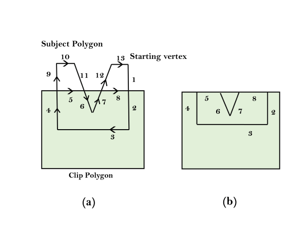
Let the clipping window be initially called clip polygon and the polygon to be clipped the subject polygon. We start with an arbitrary vertex of the subject polygon and trace around its border in the clockwise direction until an intersection with the clip polygon is encountered:

1. If the edge enters the clip polygon, record the intersection point and continue to trace the subject polygon.

2. If the edge leaves the clip polygon, record the intersection point and make a right turn to follow the clip polygon in the same manner (i.e., treat the clip polygon as subject polygon and the subject polygon as clip polygon and proceed as before).

Whenever our path of traversal forms a sub-polygon we output the sub-polygon as part of the overall result. We then continue to trace the rest of the original subject polygon from a recorded intersection point that marks the beginning of a not-yet traced edge or portion of an edge. The algorithm terminates when the entire border of the original subject polygon has been traced exactly once.

For example, the number in fig (a) indicates the order in which the edges and portion of edges are traced. We begin at the starting vertex and continue along the same edge (from 1 to 2) of the subject polygon as it enters the clip polygon. As we move along the edge that is leaving the clip polygon, we make a right turn (from 4 to 5) onto the clip polygon, which is now considered the subject polygon. Following the same logic leads to the next right turn (from 5 to 6) onto the current clip polygon, this is the original subject polygon. With the next step done (from 7 to 8) in the same way, we have a sub-polygon for output in fig (b). We then resume our traversal of the original subject polygon from the recorded intersection point where we first changed our course. Going from 9 to 10 to 11 produces no output. After skipping the already traversed 6 and 7, we continue with 12 and 13 and come to an end. The fig (b) is the final result.

Sutherland –hodgeman polygon clipping algorithm

Polygon:

Polygon is a representation of the surface. It is primitive which is closed in nature. It is formed using a collection of lines. It is also called as many-sided figure. The lines combined to form polygon are called sides or edges. The lines are obtained by combining two vertices.

Types of Polygons

1. Concave
2. Convex

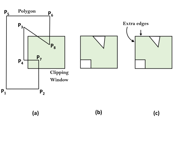
A polygon is called convex of line joining any two interior points of the polygon lies inside the polygon. A non-convex polygon is said to be concave. A concave polygon has one interior angle greater than 180°. So that it can be clipped into similar polygons. 

Sutherland –hodgeman polygon clipping algorithm

---

Introduction: We can correctly clip a polygon by processing the polygon boundary as a whole against each window edge. This could be accomplished by processing all polygon vertices against each clip rectangle boundary in turn. Beginning with the initial set of polygon vertices, we could first clip the polygon against the left rectangle boundary to produce a new sequence of vertices. The new set of vertices could then k successively passed to a right boundary clipper, a bottom boundary clipper, and a top boundary clipper, as in Fig. 6-19. At each step, a new sequence of output vertices is generated and passed to the next window boundary clipper.

It is often necessary, particularly in graphics applications, to "clip" a given polygon with another. Figure 1 shows an example. In the figure, the clipping polygon is drawn with a dashed line, the clipped polygon with a regular line, and the resulting polygon is drawn with a heavy line. In this article we'll look at the particular case where the clipping polygon is a rectangle which is oriented parallel with the axes. For this case, the Sutherland-Hodgeman algorithm is often employed. This is the algorithm that we will explore.

 

 

The Sutherland-Hodgeman Algorithm

The Sutherland-Hodgeman polygon clipping algorithm is relatively straightforward and is easily implemented in C. It does have some limitations, which we'll explore later. First, let's see how it works. For each of the four sides of the clipping rectangle, consider the line L through the two points which define that side. For each side, this line creates two planes, one which includes the clipping rectangle and one which does not. We'll call the one which does not the "clipping plane" (Figure 2).

 

 

For each of the four clipping planes, we must remove any vertices of the clipped polygon which lie inside the plane and create new points where the segments associated with these vertices cross the lineL (Figure 3).

After clipping each of the four planes, we are left with the clipped polygon.

Limitations :   

This algorithm always produces a single output polygon, even if the clipped polygon is concave and arranged in such a way that multiple output polygons might reasonably be expected. Instead, the polygons will be linked with overlapping segments along the edge of the clipping rectangle (Figure 4). This may or may not be the desired result, depending on your application

In some applications, it is often necessary to clip lines against arbitrarily shaped polygons. Algorithms based on parametric line equations, such as the Liang-Barsky method and the earlier Cyrus-Beck approach, can be extended easily convex polygon windows. We do this by modifying the algorithm to include the parametric equations for the boundaries oi the clip region. Preliminary screening of line segments can be accomplished by processing lines against the coordinate extents of the clipping polygon. For concave polygon-clipping regions, we can still apply these parametric clipping procedures if we first split the concave polygon into a set of convex polygons.

Circles or other curved-boundary clipping regions are also possible, but less commonly used. Clipping algorithms far these areas are slower because intersection calculations involve nonlinear curve equations. At the first step, lines can be clipped against the bounding rectangle (coordinate extents! of the curved clip ping region. Lines that can be identified as completely outside the bounding rectangle are discarded. To identify inside lines, we can calculate the distance of line endpoints from the circle center. If the square of this distance for both endpoints of a line 1s less than or equal to the radius squared, we can save the entire line. The remaining lines arc then processed through the intersection calculations, which must solve simultaneous circle-line equations

Splitting Concave Polygons:

We can identify a concave polygon by calculating the cross products of successive edge vectors in order around the polygon perimeter. If the z component ofsome cross products is positive while others have a negative z component, we have a concave polygon. Otherwise, the polygon is convex. This is assuming that no series of three successive vertices are collinear, in which case the cross product of the two edge vectors for these vertices is zero. If all vertices are collinear, we have a degenerate polygon (a straight line). Figure 6-14 illustrates the edge vector cross-product method for identifying concave polygons.

A vector method for splitting a concave polygon in the xy plane is to calculate the edge-vector cross products in a counterclockwise order and to note the sign of the z component of the cross products. If any z component turns out to be negative (as in Fig. 6-141, the polygon is concave and we can split ~t along the line of the first edge vector in the crossproduct pair. The following example illustrates this method for splitting a concave polygon.

Liang-Barsky Line Clipping Algorithm

The Liang-Barsky algorithm is a line clipping algorithm. This algorithm is more efficient than Cohen–Sutherland line clipping algorithm and can be extended to 3-Dimensional clipping. This algorithm is considered to be the faster parametric line-clipping algorithm. The following concepts are used in this clipping:

 

1. The parametric equation of the line.
2. The inequalities describing the range of the clipping window which is used to determine the intersections between the line and the clip window.

The parametric equation of a line can be given by,

 

X = x1 + t(x2-x1)

Y = y1 + t(y2-y1)

Where, t is between 0 and 1. 

Then, writing the point-clipping conditions in the parametric form:

xwmin<= x1 + t(x2-x1) <= xwmax

ywmin<= y1 + t(y2-y1) <= ywmax

 

The above 4 inequalities can be expressed as,

tpk<= qk

 

Where k = 1, 2, 3, 4 (correspond to the left, right, bottom, and top boundaries, respectively).

 

The p and q are defined as,

p1 = -(x2-x1),  q1 = x1 - xwmin (Left Boundary) 

p2 =  (x2-x1),  q2 = xwmax - x1 (Right Boundary)

p3 = -(y2-y1),  q3 = y1 - ywmin (Bottom Boundary) 

p4 =  (y2-y1),  q4 = ywmax - y1 (Top Boundary)  

 

When the line is parallel to a view window boundary, the p value for that boundary is zero.

When pk < 0, as t increase line goes from the outside to inside (entering).

When pk > 0, line goes from inside to outside (exiting).

When pk = 0 and qk < 0 then line is trivially invisible because it is outside view window.
When pk = 0 and qk > 0 then the line is inside the corresponding window boundary.

Using the following conditions, the position of line can be determined:

 

CONDITION	POSITION OF LINE
pk = 0	parallel to the clipping boundaries
pk = 0 and qk < 0	completely outside the boundary
pk = 0 and qk >= 0	inside the parallel clipping boundary
pk < 0	line proceeds from outside to inside
pk > 0	line proceeds from inside to outside

Parameters t1 and t2 can be calculated that define the part of line that lies within the clip rectangle.

When,

1. pk < 0, maximum(0, qk/pk) is taken.
2. pk > 0, minimum(1, qk/pk) is taken.

If t1 > t2, the line is completely outside the clip window and it can be rejected. Otherwise, the endpoints of the clipped line are calculated from the two values of parameter t.

 

Algorithm –

 

1. Set tmin=0, tmax=1.
2. Calculate the values of t (t(left), t(right), t(top), t(bottom)),
   (i) If t <tmin ignore that and move to the next edge.
   (ii) else separate the t values as entering or exiting values using the inner product.
   (iii) If t is entering value, set tmin = t; if t is existing value, set tmax = t.
3. If tmin <tmax, draw a line from (x1 + tmin(x2-x1), y1 + tmin(y2-y1)) to (x1 + tmax(x2-x1), y1 + tmax(y2-y1))
4. If the line crosses over the window, (x1 + tmin(x2-x1), y1 + tmin(y2-y1)) and (x1 + tmax(x2-x1), y1 + tmax(y2-y1)) are the intersection point of line and edge.

This algorithm is presented in the following code. Line intersection parameters are initialised to the values t1 = 0 and t2 = 1.

Numerical :-

Given :🡪

P1  = (2,7)

P2 = (8 , 12)

(xwmin , ywmin) = (5,5)

(xwmin , ywmax) = (5,10)

xwmax,ywmin) = (10,5)
(xwmax , Ywmin) = (10, 10)

Δx = 8 – 2=6

 

Δy = 12 - 7 = 5

P1  =- Δx=-6    q1= x -xwmin = 2-5 = -3
P2 = Δx = 6q2 = Xwmax– x1 = 10 - 2 = 8
P3 = - Δy = -5      q3 = y1 -Ywmin= 7-5 = 2
P4 = Δy = 5          q4 =ywmax - Y1 = 10 - 7=3

r1  =  q1 / p1 = -3 / -6 = ½

r2 = q2 / p2 = 8/6 = 4/3

r3 = q3/p3 = 2/-5  = -2/5

r4 = q4/p4 = 3/5 = 3/5

or(pi, < 0) u1 = Max (1/2 , -2/5,07) = ½

or (pi> 0) u2 = Min(4/3 , 3/5 ,1) = 3/5

u1 < u2

x1` = x1 + u1Δx = 2 + ½ *6 = 5

x2` = x1 + u2Δx = 2 + 3/5 *6 = 5.6

y1` = y1 + u1Δy = 7 + ½ *6 = 9.5

y2` = y1 + u2Δy = 7 + 3/5 *5 = 10

Coordinate of clipped lines will be (5,9.5) and (5.6 , 10).

Q: Apply the Liang-Barsky to clip the line segment from A(3,7) to B(8,10) against the regular rectangular window P(1,2) , Q(9,2) ,

R(9,8) and S(1,8).

Ans:-                                                                    [AKTU 2014-15  7M]

(x1,y1) = (3,7)

(x2 , y2) = (8,10)

Δx = x2 – x1 = 8-3 = 5

Δy = y2 – y1 = 10-7 = 3

P1 = -Δx = -5                                    q1 = x1 - xmin = 3-1 = 2

P2 = Δx = 5                                       q2 = xmax - x1 = 9 -3 = 6

P3 = -Δy = -3                                     q3 = y1 - ymin = 7 - 2 = 5

P4 = Δy = -3                                       q4 = ymax– y1 = 8 - 7 = 1

r1 = q1/p1 = 2/-5 = -0.4

 r2 = q2/p2 = 6/5 = 1.2

r3 = q3/p3 = 5/-3 = -1.66

r4 = q4/p4 = 1/3 = 0.33

u1 = max(-0.4 , -1.66 , 0) = 0

u2 = min(1,1.2,0.33) = 0.33

u1<u2 endpoints are visible

x1` = x1 + (Δx * u1) = 3 +(5*0) = 3

y1` = y1 + (Δy * u1) = 7 +(3*0) = 7

x2` = x1 + (Δx * u2) = 3 +(5*0.33) = 4.65

y2` = y1 + (Δy * u2) = 7 +(3*0.33) = 7.99

Visible line will be P1(3,7) and P2(4.65 , 7.99).

Mid Point Subdivision Line Clipping Algorithm

It is used for clipping line. The line is divided in two parts. Mid points of line is obtained by dividing it in two short segments. Again division is done, by finding midpoint. This process is continued until line of visible and invisible category is obtained. Let (x_i,y_i) are midpoint

x₅lie on point of intersection of boundary of window.

Advantage of midpoint subdivision Line Clipping:

It is suitable for machines in which multiplication and division operation is not possible. Because it can be performed by introducing clipping divides in hardware.

Algorithm of midpoint subdivision Line Clipping:

Step1: Calculate the position of both endpoints of the line

Step2: Perform OR operation on both of these endpoints

Step3: If the OR operation gives 0000
            then
                    Line is guaranteed to be visible
          else
                  Perform AND operation on both endpoints.
                  If AND ≠ 0000
            then the line is invisible
      else
            AND=6000
            then the line is clipped case.

Step4: For the line to be clipped. Find midpoint
            X_m=(x₁+x₂)/2
            Y_m=(y₁+y₂)/2
        X_mis midpoint of X coordinate.
                  Y_mis midpoint of Y coordinate.

Step5: Check each midpoint, whether it nearest to the boundary of a window or not.

Step6: If the line is totally visible or totally rejected not found then repeat step 1 to 5.

Step7: Stop algorithm.

Example: Window size is (-3, 1) to (2, 6). A line AB is given having co-ordinates of A (-4, 2) and B (-1, 7). Does this line visible. Find the visible portion of the line using midpoint subdivision?

Solution:

Step1: Fix point A (-4, 2)

Step2: Find b"=mid of b'and b

So (-1, 5) is better than (2, 4)
Find b"&bb"(-1, 5) b (-1, 7)

      So B""to B length of line will be clipped from upper side

            Now considered left-hand side portion.

      A and B""are now endpoints

            Find mid of A and B""

      A (-4, 2) B ""(-1, 6)