πŸŽ“ Computer Science & Engineering Portal

Master Engineering Disciplines with Structured Notes

Comprehensive academic lecture notes, exam-oriented unit summaries, laboratory manuals, and previous year question papers designed strictly for university students.

πŸ“‘

University Syllabi

AKTU & AICTE aligned semester guidelines.

πŸ“

Exam Question Papers

Previous 5 years solved university papers.

πŸ’‘

Lab Manuals & Viva

Practical codes with outputs & interview Qs.

Core Subjects & Units Hub

Click on any specific unit to immediately view its lecture notes below

Viewing All Lectures

Bayesian networks

What is a Bayesian Network?

A Bayesian network falls under the category of Probabilistic Graphical Modelling technique, which is used to calculate uncertainties by using the notion of probability.

They are used to model improbability using directed acyclic graphs.

bayesian network

What is Directed Acyclic Graph?

It is used to represent the Bayesian Network. A directed acyclic graph contains nodes and links, where links denote the relationship between nodes. 

bayesian network

The node represents random variables and links define their relationship. In the diagram above, Node A and Node B are parents of Node C. This means, Node C is dependent on Node A and Node B. Likewise, Node D is the child of Node C and is dependent on Node C.

This graph can help in determining the uncertainty in an event occurring based on the conditional probability distribution of each random variable. A conditional probability table is used to represent this distribution of each variable in the network.

Let’s understand what conditional probability and joint probability are.

Joint Probability β€“  It is the measure of two events happening at the same time. It can be written as P(A∩B) 

Conditional Probability– It is the measure of the probability of an event occurring given that another event has occurred. In other terms, the conditional probability of an event X is the probability that the event will occur given that event Y has already occurred.

P(X|Y): Probability of event X occurring given that event Y already occurred.

If X and Y are dependent events, then P(X|Y) = P(X∩Y)/P(Y)

If X and Y are independent events, then P(X∩Y) = 0

So, P(X|Y) = P(X)

Let’s understand the Bayesian network by an example.

Example of Bayesian Network

bayesian network

In the above diagram, water spray and rain is the child of season, i.e., they are dependent on the season. If the floor is wet, then we can say there is rain. At last, if the floor is slippery, then it is wet.

So, we can say that the probability of a random variable is dependent on his parents.

Application of Bayesian Network

Healthcare Industry: The Bayesian network is used in the healthcare industry for the detection and prevention of diseases. Based on models built, we can find out the likely symptoms and predict whether a person will be diseased or not. For instance, if a person has cholesterol, then there are high chances that the person gets a heart problem. With this information, a person can take preventive measures.

Web Search: Bayesian Network modes can be used for search accuracy based on user intent. Based on the user’s intent, these models show things that are relevant to the person. For instance, when we search for Python functions most of the time, then the web search model activates our intent and it makes sure to show relevant things to the user.

Mail Spam Filtering: Gmail is using Bayesian Models to filter the mails by reading or understanding the context of mail. For instance, we may have observed spam emails in the spam folder in Gmail. So, how are these emails classified as spams?  Using the Bayesian model, which observes the mail and based on the previous experience and the probability it classifies mail as spam or not.

Biomonitoring: Bayesian Models are used to quantify the concentration of chemicals in blood and human tissues. These use indicators to measure blood and urine. To find the level of ECCs, one can conduct biometric studies.

Information Retrieval: Models can be used for retrieving information from the database. During this process, we refine our problem multiple times. It is used to reduce information overload.

Labels: ,

Data Science Vs Machine Learning

S.No

Data Science

Machine Learning

1.

Data Science is a field about processes and systems to extract data from structured and semi-structured data.

Machine Learning is a field of study that gives computers the capability to learn without being explicitly programmed.

2.

Need the entire analytics universe.

Combination of Machine and Data Science.

3.

Branch that deals with data.

Machines utilize data science techniques to learn about the data.

4.

Data in Data Science maybe or maybe not evolved from a machine or mechanical process.

It uses various techniques like regression and supervised clustering. 
 

5.

Data Science as a broader term not only focuses on algorithms statistics but also takes care of the data processing.

But it is only focused on algorithm statistics.

6.

It is a broad term for multiple disciplines.

It fits within data science.

7.

Many operations of data science that is, data gathering, data cleaning, data manipulation, etc.

It is three types: Unsupervised learning, Reinforcement learning, Supervised learning.

8.

Example: Netflix uses Data Science technology.

Example: Facebook uses Machine Learning technology.

Labels: ,

Issues in Machine Learning

7 Major Challenges Faced By Machine Learning Professionals

In Machine Learning, there occurs a process of analyzing data for building or training models. It is just everywhere; from Amazon product recommendations to self-driven cars, it beholds great value throughout. As per the latest research, the global machine learning market is expected to grow by 43% by 2024. This revolution has enhanced the demand for machine learning professionals to a great extent. AI and machine learning jobs have observed a significant growth rate of 75% in the past four years, and the industry is growing continuously. A career in the Machine learning domain offers job satisfaction, excellent growth, insanely high salary, but it is a complex and challenging process. 

7-Major-Challenges-Faced-By-Machine-Learning-Professionals

There are a lot of challenges that machine learning professionals face to inculcate ML skills and create an application from scratch. What are these challenges? In this blog, we will discuss seven major challenges faced by machine learning professionals. Let’s have a look.

1. Poor Quality of Data

Data plays a significant role in the machine learning process. One of the significant issues that machine learning professionals face is the absence of good quality data. Unclean and noisy data can make the whole process extremely exhausting. We don’t want our algorithm to make inaccurate or faulty predictions. Hence the quality of data is essential to enhance the output. Therefore, we need to ensure that the process of data preprocessing which includes removing outliers, filtering missing values, and removing unwanted features, is done with the utmost level of perfection.  

2. Underfitting of Training Data

This process occurs when data is unable to establish an accurate relationship between input and output variables. It simply means trying to fit in undersized jeans. It signifies the data is too simple to establish a precise relationship. To overcome this issue:

  • Maximize the training time
  • Enhance the complexity of the model
  • Add more features to the data
  • Reduce regular parameters
  • Increasing the training time of model

3. Overfitting of Training Data

Overfitting refers to a machine learning model trained with a massive amount of data that negatively affect its performance. It is like trying to fit in Oversized jeans. Unfortunately, this is one of the significant issues faced by machine learning professionals. This means that the algorithm is trained with noisy and biased data, which will affect its overall performance. Let’s understand this with the help of an example. Let’s consider a model trained to differentiate between a cat, a rabbit, a dog, and a tiger. The training data contains 1000 cats, 1000 dogs, 1000 tigers, and 4000 Rabbits. Then there is a considerable probability that it will identify the cat as a rabbit. In this example, we had a vast amount of data, but it was biased; hence the prediction was negatively affected.  

We can tackle this issue by:

  • Analyzing the data with the utmost level of perfection
  • Use data augmentation technique
  • Remove outliers in the training set
  • Select a model with lesser features

4. Machine Learning is a Complex Process

The machine learning industry is young and is continuously changing. Rapid hit and trial experiments are being carried on. The process is transforming, and hence there are high chances of error which makes the learning complex. It includes analyzing the data, removing data bias, training data, applying complex mathematical calculations, and a lot more. Hence it is a really complicated process which is another big challenge for Machine learning professionals.

5. Lack of Training Data

The most important task you need to do in the machine learning process is to train the data to achieve an accurate output. Less amount training data will produce inaccurate or too biased predictions. Let us understand this with the help of an example. Consider a machine learning algorithm similar to training a child. One day you decided to explain to a child how to distinguish between an apple and a watermelon. You will take an apple and a watermelon and show him the difference between both based on their color, shape, and taste. In this way, soon, he will attain perfection in differentiating between the two. But on the other hand, a machine-learning algorithm needs a lot of data to distinguish. For complex problems, it may even require millions of data to be trained. Therefore we need to ensure that Machine learning algorithms are trained with sufficient amounts of data.

6. Slow Implementation

This is one of the common issues faced by machine learning professionals. The machine learning models are highly efficient in providing accurate results, but it takes a tremendous amount of time. Slow programs, data overload, and excessive requirements usually take a lot of time to provide accurate results. Further, it requires constant monitoring and maintenance to deliver the best output.

7. Imperfections in the Algorithm When Data Grows

So you have found quality data, trained it amazingly, and the predictions are really concise and accurate. Yay, you have learned how to create a machine learning algorithm!!  But wait, there is a twist; the model may become useless in the future as data grows. The best model of the present may become inaccurate in the coming Future and require further rearrangement. So you need regular monitoring and maintenance to keep the algorithm working. This is one of the most exhausting issues faced by machine learning professionals.

Labels: ,

Genetic Algorithms

Genetic Algorithms

Genetic Algorithms(GAs) are adaptive heuristic search algorithms that belong to the larger part of evolutionary algorithms. Genetic algorithms are based on the ideas of natural selection and genetics. These are intelligent exploitation of random search provided with historical data to direct the search into the region of better performance in solution space. They are commonly used to generate high-quality solutions for optimization problems and search problems.

Genetic algorithms simulate the process of natural selection which means those species who can adapt to changes in their environment are able to survive and reproduce and go to next generation. In simple words, they simulate β€œsurvival of the fittest” among individual of consecutive generation for solving a problem. Each generation consist of a population of individuals and each individual represents a point in search space and possible solution. Each individual is represented as a string of character/integer/float/bits. This string is analogous to the Chromosome.

Foundation of Genetic Algorithms

Genetic algorithms are based on an analogy with genetic structure and behavior of chromosomes of the population. Following is the foundation of GAs based on this analogy –  


  1. Individual in population compete for resources and mate
  2. Those individuals who are successful (fittest) then mate to create more offspring than others
  3. Genes from β€œfittest” parent propagate throughout the generation, that is sometimes parents create offspring which is better than either parent.
  4. Thus each successive generation is more suited for their environment.

Search space

The population of individuals are maintained within search space. Each individual represents a solution in search space for given problem. Each individual is coded as a finite length vector (analogous to chromosome) of components. These variable components are analogous to Genes. Thus a chromosome (individual) is composed of several genes (variable components). 

Fitness Score

A Fitness Score is given to each individual which shows the ability of an individual to β€œcompete”. The individual having optimal fitness score (or near optimal) are sought. 

The GAs maintains the population of n individuals (chromosome/solutions) along with their fitness scores.The individuals having better fitness scores are given more chance to reproduce than others. The individuals with better fitness scores are selected who mate and produce better offspring by combining chromosomes of parents. The population size is static so the room has to be created for new arrivals. So, some individuals die and get replaced by new arrivals eventually creating new generation when all the mating opportunity of the old population is exhausted. It is hoped that over successive generations better solutions will arrive while least fit die. 

Each new generation has on average more β€œbetter genes” than the individual (solution) of previous generations. Thus each new generations have better β€œpartial solutions” than previous generations. Once the offsprings produced having no significant difference than offspring produced by previous populations, the population is converged. The algorithm is said to be converged to a set of solutions for the problem.

Operators of Genetic Algorithms


Once the initial generation is created, the algorithm evolve the generation using following operators – 
1) Selection Operator: The idea is to give preference to the individuals with good fitness scores and allow them to pass there genes to successive generations. 
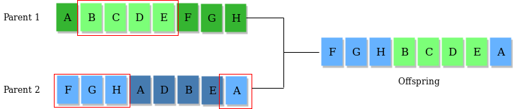
2) Crossover Operator: This represents mating between individuals. Two individuals are selected using selection operator and crossover sites are chosen randomly. Then the genes at these crossover sites are exchanged thus creating a completely new individual (offspring). For example – 

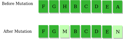
3) Mutation Operator: The key idea is to insert random genes in offspring to maintain the diversity in the population to avoid premature convergence. For example – 
 

The whole algorithm can be summarized as –  

1) Randomly initialize populations p
2) Determine fitness of population
3) Until convergence repeat:
a) Select parents from population
b) Crossover and generate new population
c) Perform mutation on new population
d) Calculate fitness for new population

Example problem and solution using Genetic Algorithms

Given a target string, the goal is to produce target string starting from a random string of the same length. In the following implementation, following analogies are made – 

  • Characters A-Z, a-z, 0-9, and other special symbols are considered as genes
  • A string generated by these characters is considered as chromosome/solution/Individual

Fitness score is the number of characters which differ from characters in target string at a particular index. So individual having lower fitness value is given more preference.  

Labels: ,

Support Vector Machine Algorithm

Support Vector Machine Algorithm

Support Vector Machine or SVM is one of the most popular Supervised Learning algorithms, which is used for Classification as well as Regression problems. However, primarily, it is used for Classification problems in Machine Learning.

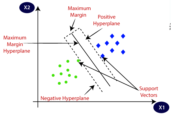
The goal of the SVM algorithm is to create the best line or decision boundary that can segregate n-dimensional space into classes so that we can easily put the new data point in the correct category in the future. This best decision boundary is called a hyperplane.

SVM chooses the extreme points/vectors that help in creating the hyperplane. These extreme cases are called as support vectors, and hence algorithm is termed as Support Vector Machine. Consider the below diagram in which there are two different categories that are classified using a decision boundary or hyperplane:

Support Vector Machine Algorithm

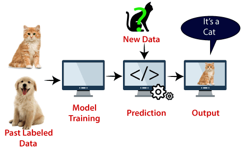
Example: SVM can be understood with the example that we have used in the KNN classifier. Suppose we see a strange cat that also has some features of dogs, so if we want a model that can accurately identify whether it is a cat or dog, so such a model can be created by using the SVM algorithm. We will first train our model with lots of images of cats and dogs so that it can learn about different features of cats and dogs, and then we test it with this strange creature. So as support vector creates a decision boundary between these two data (cat and dog) and choose extreme cases (support vectors), it will see the extreme case of cat and dog. On the basis of the support vectors, it will classify it as a cat. Consider the below diagram:

Support Vector Machine Algorithm

SVM algorithm can be used for Face detection, image classification, text categorization, etc.

Labels: ,

Decision Tree Learning

Decision Tree Classification Algorithm

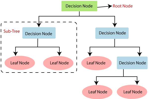
  • Decision Tree is a Supervised learning technique that can be used for both classification and Regression problems, but mostly it is preferred for solving Classification problems. It is a tree-structured classifier, where internal nodes represent the features of a dataset, branches represent the decision rules and each leaf node represents the outcome.
  • In a Decision tree, there are two nodes, which are the Decision Node and Leaf Node. Decision nodes are used to make any decision and have multiple branches, whereas Leaf nodes are the output of those decisions and do not contain any further branches.
  • The decisions or the test are performed on the basis of features of the given dataset.
  • It is a graphical representation for getting all the possible solutions to a problem/decision based on given conditions.
  • It is called a decision tree because, similar to a tree, it starts with the root node, which expands on further branches and constructs a tree-like structure.
  • In order to build a tree, we use the CART algorithm, which stands for Classification and Regression Tree algorithm.
  • A decision tree simply asks a question, and based on the answer (Yes/No), it further split the tree into subtrees.
  • Below diagram explains the general structure of a decision tree:

Note: A decision tree can contain categorical data (YES/NO) as well as numeric data.

Decision Tree Classification Algorithm

Why use Decision Trees?

There are various algorithms in Machine learning, so choosing the best algorithm for the given dataset and problem is the main point to remember while creating a machine learning model. Below are the two reasons for using the Decision tree:

  • Decision Trees usually mimic human thinking ability while making a decision, so it is easy to understand.
  • The logic behind the decision tree can be easily understood because it shows a tree-like structure.

Decision Tree Terminologies

  • Root Node: Root node is from where the decision tree starts. It represents the entire dataset, which further gets divided into two or more homogeneous sets.
  • Leaf Node: Leaf nodes are the final output node, and the tree cannot be segregated further after getting a leaf node.
  • Splitting: Splitting is the process of dividing the decision node/root node into sub-nodes according to the given conditions.
  • Branch/Sub Tree: A tree formed by splitting the tree.
  • Pruning: Pruning is the process of removing the unwanted branches from the tree.
  • Parent/Child node: The root node of the tree is called the parent node, and other nodes are called the child nodes.
  • How does the Decision Tree algorithm Work?

    In a decision tree, for predicting the class of the given dataset, the algorithm starts from the root node of the tree. This algorithm compares the values of root attribute with the record (real dataset) attribute and, based on the comparison, follows the branch and jumps to the next node.

    For the next node, the algorithm again compares the attribute value with the other sub-nodes and move further. It continues the process until it reaches the leaf node of the tree. The complete process can be better understood using the below algorithm:

    • Step-1: Begin the tree with the root node, says S, which contains the complete dataset.
    • Step-2: Find the best attribute in the dataset using Attribute Selection Measure (ASM).
    • Step-3: Divide the S into subsets that contains possible values for the best attributes.
    • Step-4: Generate the decision tree node, which contains the best attribute.
    • Step-5: Recursively make new decision trees using the subsets of the dataset created in step -3. Continue this process until a stage is reached where you cannot further classify the nodes and called the final node as a leaf node.

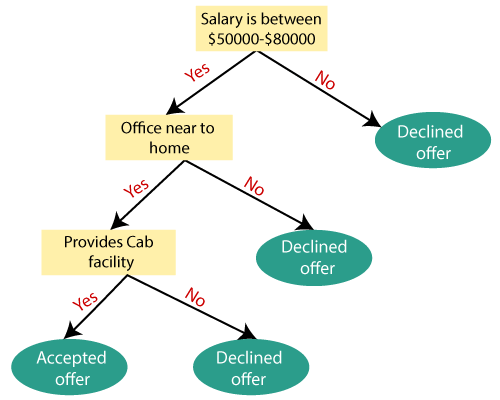
    Example: Suppose there is a candidate who has a job offer and wants to decide whether he should accept the offer or Not. So, to solve this problem, the decision tree starts with the root node (Salary attribute by ASM). The root node splits further into the next decision node (distance from the office) and one leaf node based on the corresponding labels. The next decision node further gets split into one decision node (Cab facility) and one leaf node. Finally, the decision node splits into two leaf nodes (Accepted offers and Declined offer). Consider the below diagram:

    Decision Tree Classification Algorithm


    Labels: ,

    Reinforcement learning

    Reinforcement learning

    Reinforcement learning is an area of Machine Learning. It is about taking suitable action to maximize reward in a particular situation. It is employed by various software and machines to find the best possible behavior or path it should take in a specific situation. Reinforcement learning differs from supervised learning in a way that in supervised learning the training data has the answer key with it so the model is trained with the correct answer itself whereas in reinforcement learning, there is no answer but the reinforcement agent decides what to do to perform the given task. In the absence of a training dataset, it is bound to learn from its experience. 

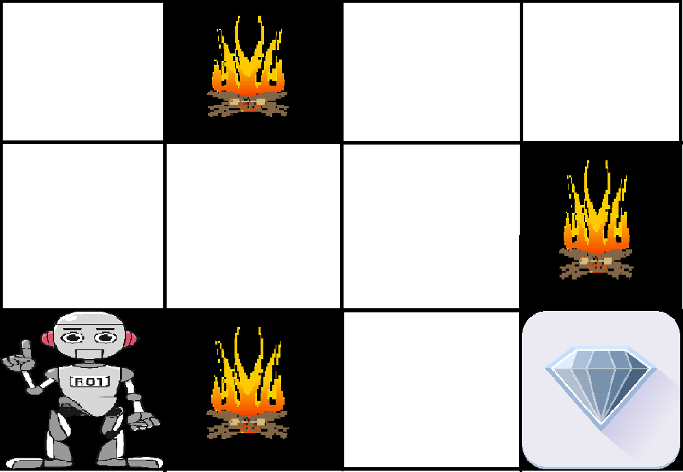
    Example: The problem is as follows: We have an agent and a reward, with many hurdles in between. The agent is supposed to find the best possible path to reach the reward. The following problem explains the problem more easily. 


    The above image shows the robot, diamond, and fire. The goal of the robot is to get the reward that is the diamond and avoid the hurdles that are fired. The robot learns by trying all the possible paths and then choosing the path which gives him the reward with the least hurdles. Each right step will give the robot a reward and each wrong step will subtract the reward of the robot. The total reward will be calculated when it reaches the final reward that is the diamond. 

    Main points in Reinforcement learning –  

    • Input: The input should be an initial state from which the model will start
    • Output: There are many possible outputs as there are a variety of solutions to a particular problem
    • Training: The training is based upon the input, The model will return a state and the user will decide to reward or punish the model based on its output.
    • The model keeps continues to learn.
    • The best solution is decided based on the maximum reward.

    Difference between Reinforcement learning and Supervised learning: 

    Types of Reinforcement: There are two types of Reinforcement:  

    1. Positive – 
      Positive Reinforcement is defined as when an event, occurs due to a particular behavior, increases the strength and the frequency of the behavior. In other words, it has a positive effect on behavior. 

      Advantages of reinforcement learning are: 

      • Maximizes Performance
      • Sustain Change for a long period of time
      • Too much Reinforcement can lead to an overload of states which can diminish the results
    2. Negative – 
      Negative Reinforcement is defined as strengthening of behavior because a negative condition is stopped or avoided. 

      Advantages of reinforcement learning: 

      • Increases Behavior
      • Provide defiance to a minimum standard of performance
      • It Only provides enough to meet up the minimum behavior

    Various Practical applications of Reinforcement Learning –  

    • RL can be used in robotics for industrial automation.
    • RL can be used in machine learning and data processing
    • RL can be used to create training systems that provide custom instruction and materials according to the requirement of students.

    RL can be used in large environments in the following situations:  

    1. A model of the environment is known, but an analytic solution is not available;
    2. Only a simulation model of the environment is given (the subject of simulation-based optimization)
    3. The only way to collect information about the environment is to interact with it.

    Labels: ,

    Clustering

    Clustering

    Clustering or cluster analysis is a machine learning technique, which groups the unlabelled dataset. It can be defined as "A way of grouping the data points into different clusters, consisting of similar data points. The objects with the possible similarities remain in a group that has less or no similarities with another group."

    It does it by finding some similar patterns in the unlabelled dataset such as shape, size, color, behavior, etc., and divides them as per the presence and absence of those similar patterns.

    It is an unsupervised learning

    method, hence no supervision is provided to the algorithm, and it deals with the unlabeled dataset.

    After applying this clustering technique, each cluster or group is provided with a cluster-ID. ML system can use this id to simplify the processing of large and complex datasets.

    The clustering technique is commonly used for statistical data analysis.

    Note: Clustering is somewhere similar to the classification algorithm
    , but the difference is the type of dataset that we are using. In classification, we work with the labeled data set, whereas in clustering, we work with the unlabelled dataset.

    Example: Let's understand the clustering technique with the real-world example of Mall: When we visit any shopping mall, we can observe that the things with similar usage are grouped together. Such as the t-shirts are grouped in one section, and trousers are at other sections, similarly, at vegetable sections, apples, bananas, Mangoes, etc., are grouped in separate sections, so that we can easily find out the things. The clustering technique also works in the same way. Other examples of clustering are grouping documents according to the topic.

    The clustering technique can be widely used in various tasks. Some most common uses of this technique are:

    • Market Segmentation
    • Statistical data analysis
    • Social network analysis
    • Image segmentation
    • Anomaly detection, etc.

    Apart from these general usages, it is used by the Amazon in its recommendation system to provide the recommendations as per the past search of products. Netflix also uses this technique to recommend the movies and web-series to its users as per the watch history.

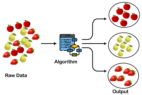
    The below diagram explains the working of the clustering algorithm. We can see the different fruits are divided into several groups with similar properties.
    Clustering in Machine Learning

    Types of Clustering Methods

    The clustering methods are broadly divided into Hard clustering (datapoint belongs to only one group) and Soft Clustering (data points can belong to another group also). But there are also other various approaches of Clustering exist. Below are the main clustering methods used in Machine learning:

    1. Partitioning Clustering
    2. Density-Based Clustering
    3. Distribution Model-Based Clustering
    4. Hierarchical Clustering
    5. Fuzzy Clustering

    Partitioning Clustering

    It is a type of clustering that divides the data into non-hierarchical groups. It is also known as the centroid-based method. The most common example of partitioning clustering is the K-Means Clustering algorithm

    .

    In this type, the dataset is divided into a set of k groups, where K is used to define the number of pre-defined groups. The cluster center is created in such a way that the distance between the data points of one cluster is minimum as compared to another cluster centroid.
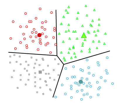
    Clustering in Machine Learning

    Density-Based Clustering

    The density-based clustering method connects the highly-dense areas into clusters, and the arbitrarily shaped distributions are formed as long as the dense region can be connected. This algorithm does it by identifying different clusters in the dataset and connects the areas of high densities into clusters. The dense areas in data space are divided from each other by sparser areas.

    These algorithms can face difficulty in clustering the data points if the dataset has varying densities and high dimensions.
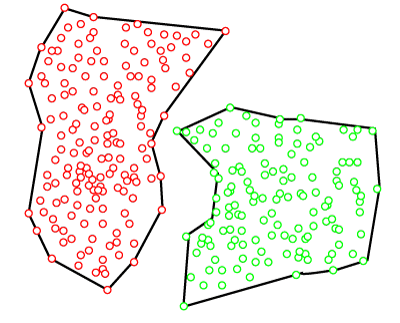
    Clustering in Machine Learning

    Distribution Model-Based Clustering

    In the distribution model-based clustering method, the data is divided based on the probability of how a dataset belongs to a particular distribution. The grouping is done by assuming some distributions commonly Gaussian Distribution.

    The example of this type is the Expectation-Maximization Clustering algorithm that uses Gaussian Mixture Models (GMM).
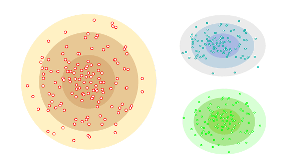
    Clustering in Machine Learning

    Hierarchical Clustering

    Hierarchical clustering can be used as an alternative for the partitioned clustering as there is no requirement of pre-specifying the number of clusters to be created. In this technique, the dataset is divided into clusters to create a tree-like structure, which is also called a dendrogram. The observations or any number of clusters can be selected by cutting the tree at the correct level. The most common example of this method is the Agglomerative Hierarchical algorithm.
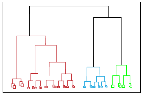
    Clustering in Machine Learning

    Fuzzy Clustering

    Fuzzy

    clustering is a type of soft method in which a data object may belong to more than one group or cluster. Each dataset has a set of membership coefficients, which depend on the degree of membership to be in a cluster. Fuzzy C-means algorithm is the example of this type of clustering; it is sometimes also known as the Fuzzy k-means algorithm.

    Clustering Algorithms

    The Clustering algorithms can be divided based on their models that are explained above. There are different types of clustering algorithms published, but only a few are commonly used. The clustering algorithm is based on the kind of data that we are using. Such as, some algorithms need to guess the number of clusters in the given dataset, whereas some are required to find the minimum distance between the observation of the dataset.

    Here we are discussing mainly popular Clustering algorithms that are widely used in machine learning:

    1. K-Means algorithm: The k-means algorithm is one of the most popular clustering algorithms. It classifies the dataset by dividing the samples into different clusters of equal variances. The number of clusters must be specified in this algorithm. It is fast with fewer computations required, with the linear complexity of O(n).
    2. Mean-shift algorithm: Mean-shift algorithm tries to find the dense areas in the smooth density of data points. It is an example of a centroid-based model, that works on updating the candidates for centroid to be the center of the points within a given region.
    3. DBSCAN Algorithm: It stands for Density-Based Spatial Clustering of Applications with Noise. It is an example of a density-based model similar to the mean-shift, but with some remarkable advantages. In this algorithm, the areas of high density are separated by the areas of low density. Because of this, the clusters can be found in any arbitrary shape.
    4. Expectation-Maximization Clustering using GMM: This algorithm can be used as an alternative for the k-means algorithm or for those cases where K-means can be failed. In GMM, it is assumed that the data points are Gaussian distributed.
    5. Agglomerative Hierarchical algorithm: The Agglomerative hierarchical algorithm performs the bottom-up hierarchical clustering. In this, each data point is treated as a single cluster at the outset and then successively merged. The cluster hierarchy can be represented as a tree-structure.
    6. Affinity Propagation: It is different from other clustering algorithms as it does not require to specify the number of clusters. In this, each data point sends a message between the pair of data points until convergence. It has O(N2T) time complexity, which is the main drawback of this algorithm.

    Applications of Clustering

    Below are some commonly known applications of clustering technique in Machine Learning:

    • In Identification of Cancer Cells: The clustering algorithms are widely used for the identification of cancerous cells. It divides the cancerous and non-cancerous data sets into different groups.
    • In Search Engines: Search engines also work on the clustering technique. The search result appears based on the closest object to the search query. It does it by grouping similar data objects in one group that is far from the other dissimilar objects. The accurate result of a query depends on the quality of the clustering algorithm used.
    • Customer Segmentation: It is used in market research to segment the customers based on their choice and preferences.
    • In Biology: It is used in the biology stream to classify different species of plants and animals using the image recognition technique.
    • In Land Use: The clustering technique is used in identifying the area of similar lands use in the GIS database. This can be very useful to find that for what purpose the particular land should be used, that means for which purpose it is more suitable.

    Labels: ,