🎓 Computer Science & Engineering Portal

Master Engineering Disciplines with Structured Notes

Comprehensive academic lecture notes, exam-oriented unit summaries, laboratory manuals, and previous year question papers designed strictly for university students.

📑

University Syllabi

AKTU & AICTE aligned semester guidelines.

📝

Exam Question Papers

Previous 5 years solved university papers.

💡

Lab Manuals & Viva

Practical codes with outputs & interview Qs.

Core Subjects & Units Hub

Click on any specific unit to immediately view its lecture notes below

Viewing All Lectures

Comparison between CLASSIFICATION, CLUSTERING and Regression

Comparison between Classification and Clustering: 

Parameter

CLASSIFICATION

CLUSTERING

Type

used for supervised learning

used for unsupervised learning

Basic

process of classifying the input instances based on their corresponding class labels

grouping the instances based on their similarity without the help of class labels

Need

it has labels so there is need of training and testing dataset for verifying the model created

there is no need of training and testing dataset

Complexity

more complex as compared to clustering

less complex as compared to classification

Example Algorithms

Logistic regression, Naive Bayes classifier, Support vector machines, etc.

k-means clustering algorithm, Fuzzy c-means clustering algorithm, Gaussian (EM) clustering algorithm, etc.

Differences between Classification and Clustering 

  1. Classification is used for supervised learning whereas clustering is used for unsupervised learning.
  2. The process of classifying the input instances based on their corresponding class labels is known as classification whereas grouping the instances based on their similarity without the help of class labels is known as clustering.
  3. As Classification have labels so there is need of training and testing dataset for verifying the model created but there is no need for training and testing dataset in clustering.
  4. Classification is more complex as compared to clustering as there are many levels in the classification phase whereas only grouping is done in clustering.
  5. Classification examples are Logistic regression, Naive Bayes classifier, Support vector machines, etc. Whereas clustering examples are k-means clustering algorithm, Fuzzy c-means clustering algorithm, Gaussian (EM) clustering algorithm, etc.

Regression vs. Classification in Machine Learning

Regression and Classification algorithms are Supervised Learning algorithms. Both the algorithms are used for prediction in Machine learning and work with the labeled datasets. But the difference between both is how they are used for different machine learning problems.

The main difference between Regression and Classification algorithms that Regression algorithms are used to predict the continuous values such as price, salary, age, etc. and Classification algorithms are used to predict/Classify the discrete values such as Male or Female, True or False, Spam or Not Spam, etc.

Consider the below diagram:
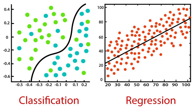
Regression vs. Classification

Classification:

Classification is a process of finding a function which helps in dividing the dataset into classes based on different parameters. In Classification, a computer program is trained on the training dataset and based on that training, it categorizes the data into different classes.

The task of the classification algorithm is to find the mapping function to map the input(x) to the discrete output(y).

Example: The best example to understand the Classification problem is Email Spam Detection. The model is trained on the basis of millions of emails on different parameters, and whenever it receives a new email, it identifies whether the email is spam or not. If the email is spam, then it is moved to the Spam folder.

Types of ML Classification Algorithms:

Classification Algorithms can be further divided into the following types:

  • Logistic Regression
  • K-Nearest Neighbours
  • Support Vector Machines
  • Kernel SVM
  • Naïve Bayes
  • Decision Tree Classification
  • Random Forest Classification

Regression:

Regression is a process of finding the correlations between dependent and independent variables. It helps in predicting the continuous variables such as prediction of Market Trends, prediction of House prices, etc.

The task of the Regression algorithm is to find the mapping function to map the input variable(x) to the continuous output variable(y).

Example: Suppose we want to do weather forecasting, so for this, we will use the Regression algorithm. In weather prediction, the model is trained on the past data, and once the training is completed, it can easily predict the weather for future days.

Types of Regression Algorithm:

  • Simple Linear Regression
  • Multiple Linear Regression
  • Polynomial Regression
  • Support Vector Regression
  • Decision Tree Regression
  • Random Forest Regression

Clustering

It is basically a type of unsupervised learning method. An unsupervised learning method is a method in which we draw references from datasets consisting of input data without labeled responses. Generally, it is used as a process to find meaningful structure, explanatory underlying processes, generative features, and groupings inherent in a set of examples. 

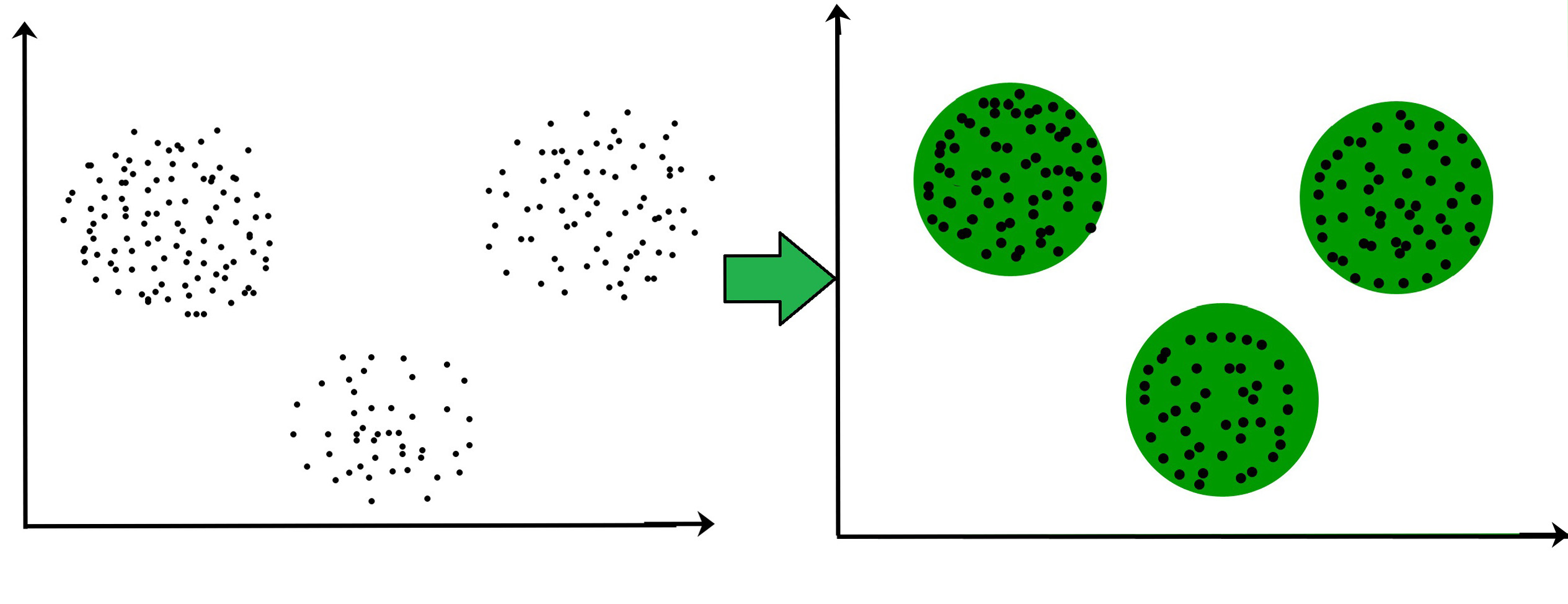
Clustering is the task of dividing the population or data points into a number of groups such that data points in the same groups are more similar to other data points in the same group and dissimilar to the data points in other groups. It is basically a collection of objects on the basis of similarity and dissimilarity between them. 


For ex– The data points in the graph below clustered together can be classified into one single group. We can distinguish the clusters, and we can identify that there are 3 clusters in the below picture. 
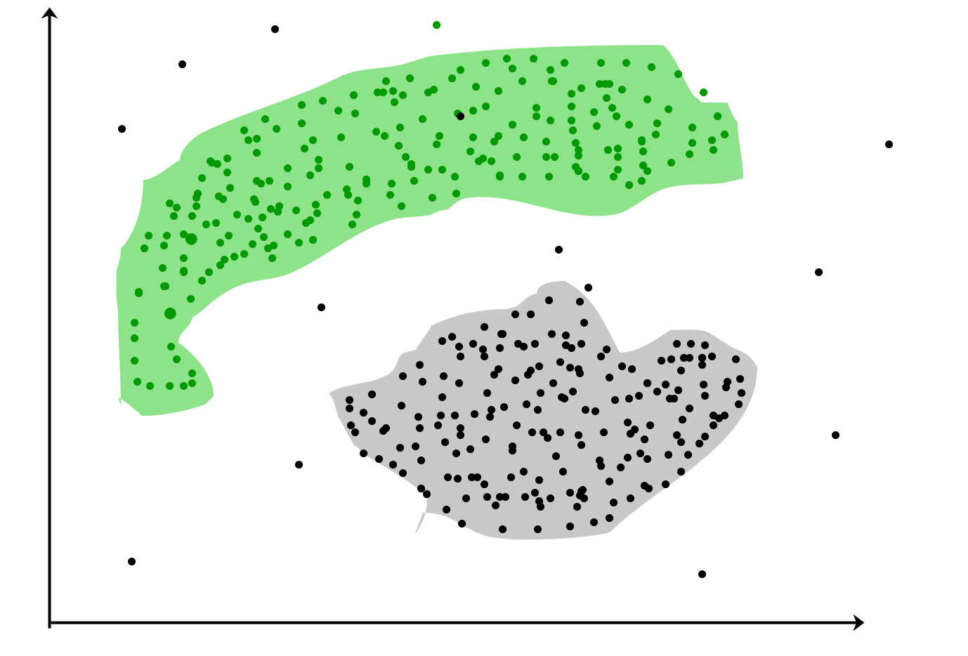
It is not necessary for clusters to be spherical. Such as : 
Difference between Regression and Classification

Regression Algorithm

Classification Algorithm

In Regression, the output variable must be of continuous nature or real value.

In Classification, the output variable must be a discrete value.

The task of the regression algorithm is to map the input value (x) with the continuous output variable(y).

The task of the classification algorithm is to map the input value(x) with the discrete output variable(y).

Regression Algorithms are used with continuous data.

Classification Algorithms are used with discrete data.

In Regression, we try to find the best fit line, which can predict the output more accurately.

In Classification, we try to find the decision boundary, which can divide the dataset into different classes.

Regression algorithms can be used to solve the regression problems such as Weather Prediction, House price prediction, etc.

Classification Algorithms can be used to solve classification problems such as Identification of spam emails, Speech Recognition, Identification of cancer cells, etc.

The regression Algorithm can be further divided into Linear and Non-linear Regression.

The Classification algorithms can be divided into Binary Classifier and Multi-class Classifier.

Labels: ,

Application of Genetic Algorithms

Genetic Algorithms are primarily used in optimization problems of various kinds, but they are frequently used in other application areas as well.

In this section, we list some of the areas in which Genetic Algorithms are frequently used. These are −

  • Optimization − Genetic Algorithms are most commonly used in optimization problems wherein we have to maximize or minimize a given objective function value under a given set of constraints. The approach to solve Optimization problems has been highlighted throughout the tutorial.

  • Economics − GAs are also used to characterize various economic models like the cobweb model, game theory equilibrium resolution, asset pricing, etc.

  • Neural Networks − GAs are also used to train neural networks, particularly recurrent neural networks.

  • Parallelization − GAs also have very good parallel capabilities, and prove to be very effective means in solving certain problems, and also provide a good area for research.

  • Image Processing − GAs are used for various digital image processing (DIP) tasks as well like dense pixel matching.

  • Vehicle routing problems − With multiple soft time windows, multiple depots and a heterogeneous fleet.

  • Scheduling applications − GAs are used to solve various scheduling problems as well, particularly the time tabling problem.

  • Machine Learning − as already discussed, genetics based machine learning (GBML) is a niche area in machine learning.

  • Robot Trajectory Generation − GAs have been used to plan the path which a robot arm takes by moving from one point to another.

  • Parametric Design of Aircraft − GAs have been used to design aircrafts by varying the parameters and evolving better solutions.

  • DNA Analysis − GAs have been used to determine the structure of DNA using spectrometric data about the sample.

  • Multimodal Optimization − GAs are obviously very good approaches for multimodal optimization in which we have to find multiple optimum solutions.

  • Traveling salesman problem and its applications − GAs have been used to solve the TSP, which is a well-known combinatorial problem using novel crossover and packing strategies.

Labels: ,

Genetic Programming

What is Genetic Programming?

Genetic programming is a technique to create algorithms that can program themselves by simulating biological breeding and Darwinian evolution. Instead of programming a model that can solve a particular problem, genetic programming only provides a general objective and lets the model figure out the details itself. The basic approach is to let the machine automatically test various simple evolutionary algorithms and then “breed” the most successful programs in new generations.

While applying the same natural selection, crossover, mutations and other reproduction approaches as evolutionary and genetic algorithms, gene programming takes the process a step further by automatically creating new models and letting the system select its own goals.

The entire process is still an area of active research. One of the biggest obstacles to widespread adoption of this genetic machine learning approach is quantifying the fitness function, i.e to what degree each new program is contributing to reaching the desired goal.

How to Set Up a Genetic Program:

To set up a basic genetic program, a human first needs to define a high-level statement of the problem through several preparatory steps:

  • Specify terminals – For example, independent variables of the problem, zero-argument functions, or random constants for each branch of program that will be go through evolution.

  • Define initial “primitive” functions for each branch of the genetic program.

  • Choose a fitness measure – this measures the fitness of individuals in the population to determine if they should reproduce.

  • Any special performance parameters for controlling the run.

  • Select termination criterion and methods for reaching the run’s goals.

From there, the program runs automatically, without requiring any training data.

A random initial population (generation 0) of simple programs will be generated based upon basic functions and terminal defined by the human.

Each program will be executed and its fitness measured from the results. The most successful or “fit” programs will be breeding stock to birth a new generation, with some new population members directly copied (reproduction), some through crossover (randomly breeding parts of the programs) and random mutations. Unlike evolutionary programming, an additional architecture-altering operation is chosen, similar to a species, to control the framework of the new generation.

These generations are repeated as necessary until the termination criterion is reached and the best program is designated as the result of the run.

Labels: ,

Genetic Algorithms

Genetic Algorithms

Genetic Algorithms(GAs) are adaptive heuristic search algorithms that belong to the larger part of evolutionary algorithms. Genetic algorithms are based on the ideas of natural selection and genetics. These are intelligent exploitation of random search provided with historical data to direct the search into the region of better performance in solution space. They are commonly used to generate high-quality solutions for optimization problems and search problems.

Genetic algorithms simulate the process of natural selection which means those species who can adapt to changes in their environment are able to survive and reproduce and go to next generation. In simple words, they simulate “survival of the fittest” among individual of consecutive generation for solving a problem. Each generation consist of a population of individuals and each individual represents a point in search space and possible solution. Each individual is represented as a string of character/integer/float/bits. This string is analogous to the Chromosome.

Foundation of Genetic Algorithms

Genetic algorithms are based on an analogy with genetic structure and behavior of chromosomes of the population. Following is the foundation of GAs based on this analogy –  

  1. Individual in population compete for resources and mate
  2. Those individuals who are successful (fittest) then mate to create more offspring than others
  3. Genes from “fittest” parent propagate throughout the generation, that is sometimes parents create offspring which is better than either parent.
  4. Thus each successive generation is more suited for their environment.

Search space

The population of individuals are maintained within search space. Each individual represents a solution in search space for given problem. Each individual is coded as a finite length vector (analogous to chromosome) of components. These variable components are analogous to Genes. Thus a chromosome (individual) is composed of several genes (variable components). 

Fitness Score

A Fitness Score is given to each individual which shows the ability of an individual to “compete”. The individual having optimal fitness score (or near optimal) are sought. 

The GAs maintains the population of n individuals (chromosome/solutions) along with their fitness scores.The individuals having better fitness scores are given more chance to reproduce than others. The individuals with better fitness scores are selected who mate and produce better offspring by combining chromosomes of parents. The population size is static so the room has to be created for new arrivals. So, some individuals die and get replaced by new arrivals eventually creating new generation when all the mating opportunity of the old population is exhausted. It is hoped that over successive generations better solutions will arrive while least fit die. 

Each new generation has on average more “better genes” than the individual (solution) of previous generations. Thus each new generations have better “partial solutions” than previous generations. Once the offspring produced having no significant difference from offspring produced by previous populations, the population is converged. The algorithm is said to be converged to a set of solutions for the problem.

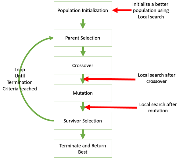
GA cycle of reproduction

Hybridize GA


Components of Genetic Algorithms

Once the initial generation is created, the algorithm evolves the generation using following operators – 
1. Crossover

The crossover operator is analogous to reproduction and biological crossover. In this more than one parent is selected and one or more off-springs are produced using the genetic material of the parents. Crossover is usually applied in a GA with a high probability – pc .

Crossover Operators

In this section we will discuss some of the most popularly used crossover operators. It is to be noted that these crossover operators are very generic and the GA Designer might choose to implement a problem-specific crossover operator as well.

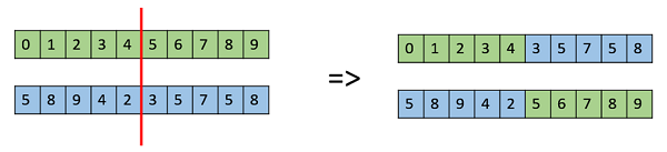
One Point Crossover

In this one-point crossover, a random crossover point is selected and the tails of its two parents are swapped to get new off-springs.

One Point Crossover

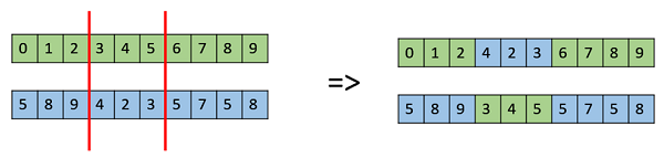
Multi Point Crossover

Multi point crossover is a generalization of the one-point crossover wherein alternating segments are swapped to get new off-springs.

Multi Point Crossover

Uniform Crossover

In a uniform crossover, we don’t divide the chromosome into segments, rather we treat each gene separately. In this, we essentially flip a coin for each chromosome to decide whether or not it’ll be included in the off-spring. We can also bias the coin to one parent, to have more genetic material in the child from that parent.

Uniform Crossover

Whole Arithmetic Recombination

This is commonly used for integer representations and works by taking the weighted average of the two parents by using the following formulae −

  • Child1 = α.x + (1-α).y
  • Child2 = α.x + (1-α).y

Obviously, if α = 0.5, then both the children will be identical as shown in the following image.

Whole Arithmetic Recombination

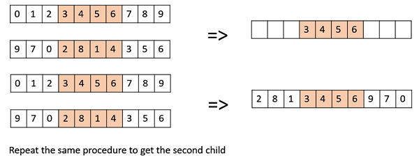
Davis’ Order Crossover (OX1)

OX1 is used for permutation based crossovers with the intention of transmitting information about relative ordering to the off-springs. It works as follows −

  • Create two random crossover points in the parent and copy the segment between them from the first parent to the first offspring.

  • Now, starting from the second crossover point in the second parent, copy the remaining unused numbers from the second parent to the first child, wrapping around the list.

  • Repeat for the second child with the parent’s role reversed.

Davis’ Order Crossover

There exist a lot of other crossovers like Partially Mapped Crossover (PMX), Order based crossover (OX2), Shuffle Crossover, Ring Crossover, etc.

 2. Mutation

In simple terms, mutation may be defined as a small random tweak in the chromosome, to get a new solution. It is used to maintain and introduce diversity in the genetic population and is usually applied with a low probability – pm. If the probability is very high, the GA gets reduced to a random search.

Mutation is the part of the GA which is related to the “exploration” of the search space. It has been observed that mutation is essential to the convergence of the GA while crossover is not.

Mutation Operators

In this section, we describe some of the most commonly used mutation operators. Like the crossover operators, this is not an exhaustive list and the GA designer might find a combination of these approaches or a problem-specific mutation operator more useful.

Bit Flip Mutation

In this bit flip mutation, we select one or more random bits and flip them. This is used for binary encoded GAs.

Bit Flip Mutation

Random Resetting

Random Resetting is an extension of the bit flip for the integer representation. In this, a random value from the set of permissible values is assigned to a randomly chosen gene.

Swap Mutation

In swap mutation, we select two positions on the chromosome at random, and interchange the values. This is common in permutation based encodings.

Swap Mutation

Scramble Mutation

Scramble mutation is also popular with permutation representations. In this, from the entire chromosome, a subset of genes is chosen and their values are scrambled or shuffled randomly.

Scramble Mutation

Inversion Mutation

In inversion mutation, we select a subset of genes like in scramble mutation, but instead of shuffling the subset, we merely invert the entire string in the subset.

Inversion Mutation


The whole algorithm can be summarized as –  

1) Randomly initialize populations p
2) Determine fitness of population
3) Until convergence repeat:
a) Select parents from population
b) Crossover and generate new population
c) Perform mutation on new population
d) Calculate fitness for new population

Example problem and solution using Genetic Algorithms

Given a target string, the goal is to produce target string starting from a random string of the same length. In the following implementation, following analogies are made – 

  • Characters A-Z, a-z, 0-9, and other special symbols are considered as genes
  • A string generated by these characters is considered as chromosome/solution/Individual

Fitness score is the number of characters which differ from characters in target string at a particular index. So individual having lower fitness value is given more preference. 

Labels: ,

Deep Q-Learning

Deep Q-Learning

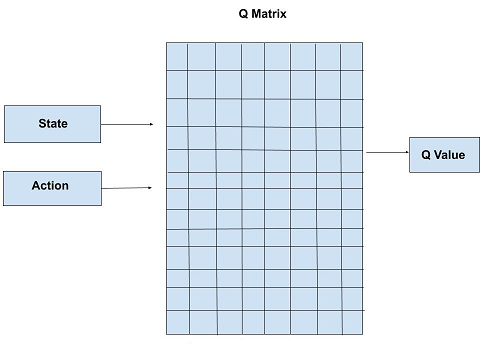
The process of Q-Learning creates an exact matrix for the working agent which it can “refer to” to maximize its reward in the long run. Although this approach is not wrong in itself, this is only practical for very small environments and quickly loses it’s feasibility when the number of states and actions in the environment increases.

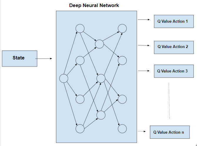
The solution for the above problem comes from the realization that the values in the matrix only have relative importance ie the values only have importance with respect to the other values. Thus, this thinking leads us to Deep Q-Learning which uses a deep neural network to approximate the values. This approximation of values does not hurt as long as the relative importance is preserved.

The basic working step for Deep Q-Learning is that the initial state is fed into the neural network and it returns the Q-value of all possible actions as on output.

The difference between Q-Learning and Deep Q-Learning can be illustrated as follows:-

Pseudo Code:

Initialize Q_{0}(s,a) for all pairs (s,a)
s = initial state
k = 0
while(convergence is not achieved)
{
simulate action a and reach state s'
if(s' is a terminal state)
{
target = R(s,a,s')
}
else
{
target = R(s,a,s') + \gamma max_{a'}Q_{k}(s',a')
}
\theta _{k+1} = \theta _{k}-\alpha \Delta _{\theta }E_{s'~P(s'|s,a)}[(Q_{\theta }(s,a)-target(s'))^{2}]|_{\theta = \theta _{k}}
s = s'
}

Observe that in the equation target = R(s,a,s’) + \gamma max_{a'}Q_{k}(s',a'), the term
\gamma max_{a'}Q_{k}(s',a') is a variable term. Therefore in this process, the target for the neural network is variable unlike other typical Deep Learning processes where the target is stationary.

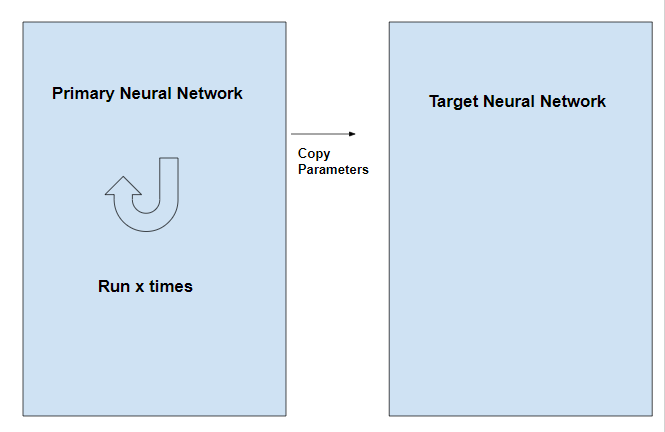
This problem is overcome by having two neural networks instead of one. One neural network is used to adjust the parameters of the network and the other is used for computing the target and which has the same architecture as the first network but has frozen parameters. After an x number of iterations in the primary network, the parameters are copied to the target network.

Labels: ,