Multiplexing

The set of techniques that allows the simultaneous transmission of multiple signals across a single data link is commonly referred to as Multiplexing. Multiplexing is done by using the hardware that is called as Multiplexer(MUX).

The Multiplexer(MUX) mainly combines 'n' input lines in order to generate '1' output line(this is simply many-to-one) on the sender side. And on the receiver side, this stream is fed into the demultiplexer(DEMUX), which then separates the stream back to its component transmission (this is one-to-many) and then directs them to their corresponding lines.

The main aim of the multiplexing technique is to share scarce resources.

Let us understand with the help of a diagram given below to divide 1 link into n channels:

In the above diagram, the word link refers to the physical path, and the word channel simply refers to the portion of the link that carries a transmission between a given pair of lines. Thus 1 link can have many channels.

History of the Multiplexing

In telecommunications, several telephone calls may be carried by using a single wire. Also, Multiplexing was originated in telegraphy in the 1870s. Now, this technique is widely applied in communications. George Owen Squier in telephony was credited with the development of telephone carrier multiplexing in the year 1910.

Need for the Multiplexing

As we have already told you that multiplexing is basically a set of techniques that mainly allows the transmission of multiple signals simultaneously across a signals data link.

At the time when there is a need to transmit many signals from the sender side that sends simultaneously then multiplexer is used to convert many signals into one so that on the receiving end we can get them simultaneously.

As it is very expensive to send many signals differently and it also requires more wires to send. Thus there is a need for multiplexing. Let us take an example of T.V cable distributor who sends many channels through a single wire.

Advantages of Multiplexing

Given below are some advantages of using Multiplexing:

• With the help of multiplexing, more than one signal can be sent easily over a single medium or link.

• Multiplexing helps in the effective utilization of the bandwidth of the medium.

Let us take a look at the given below figure to understand multiplexing vs no-multiplexing:

Categories of Multiplexing

Let us take a look at the different categories of Multiplexing:

• Frequency-division multiplexing

• Wavelength-division multiplexing

• Time-division multiplexing

Let us discuss all the above-given categories one by one in the following sections.

1. Frequency-Division Multiplexing

Frequency-Divison Multiplexing i.e FDM is an analog technique.

• With this technique, signals having different frequencies are combined in a composite signal and then transmitted on the link

• It is mainly applied at the time when the bandwidth of the link is greater than the combined bandwidths of the signal to be transmitted.

• In this, each signal is of a different frequency.

• The channel is usually separated by the strips of unused bandwidth that is the guard bands in order to prevent the signals from overlapping.

• In the case of frequency division multiplexing, suppose the input signal is in the digital form then it must be converted to analog before giving it as the input to the modulator.

Frequency Division Multiplexing

From the above diagram, in FDM the transmission path is divided into three parts and each part mainly represents a channel that carries one transmission.

Advantages

Given below are some advantages of using FDM:

• The Simultaneous transmission of a large number of signals is done easily.

• The demodulation of FDM multiplexing is easy.

• There is no need for synchronization between the transmitter and receiver for proper operation.

• In the case of slow narrowband fading, there is only one single channel that gets affected.

Disadvantages

There are some drawbacks of using FDM:

• Communication channels must have a very large bandwidth.

• There occurs the problem of crosstalk while using FDM.

• In the case of wideband fading, all channels in the FDM gets affected.

• There is a need for a large number of filters and modulators.

Applications

The main applications of FDM are as follows:

• One of the main applications of FDM is that it is AM and FM radio broadcasting.

• Another application of FDM is that it is used in television broadcasting.

• FDM is also used by first-generation cellular telephones.

2.Wavelength-Division Multiplexing

Wavelength-Divison Multiplexing i.e WDM is an analog technique.

• This technique is similar to FDM.

• With the help of Wavelength Divison multiplexing different signals that include: optical or light signals are transmitted through the Optical fiber.

• With the help of the WDM technique, the high data rate capability of optical fiber cable gets utilized.

• With this technique, various light waves from different sources are combined into a composite light signal and this signal is transmitted across the channel to the receiver.

• On the receiver side, this composite light signal gets broken down into different light waves with the help of Demultiplexer.

• The process of combining and splitting the light waves is done with the help of Prism.

• This Prism helps to bend the beam of light on the basis of the angle of incidence and frequency of light.

• In the WDM technique mainly the role of the multiplexer is played by the Prism and it then combines the various optical signals in the order to form a composite signal after that this composite signal is transmitted through an Optical fiber cable.

The above Figure indicates Wavelength Divison Multiplexing

Let us take a look at the diagram given below where we will use prism for wavelength-division multiplexing and demultiplexing.

Advantages

Given below are some advantages of using WDM:

• With the help of WDM, the full-duplex transmission is possible.

• WDM is easy to reconfigure.

• Various Signals can be transmitted simultaneously with the help of WDM.

• This technique is less expensive and the expansion of the system is easy.

• This technique provides high security.

• As we are using an optical fiber in WDM; also Optical components are more reliable and they also provide high bandwidth.

Disadvantages

There are some drawbacks of using WDM:

• There is the use of optical equipment so cost increases.

• Utilization of bandwidth can be inefficient which causes difficulty in wavelength tuning.

• The main concern in this technique is scalability.

3.Time-Division Multiplexing

Time-Divison multiplexing is a digital technique for multiplexing.

• In this technique, the channel/link is divided on the basis of time instead of frequency.

• The total available time on the channel is divided between the different users on the channel.

• A particular time interval is allotted to each user on the channel and it is known as time slot/slice.

• In the time-division multiplexing, the data rate capacity should be much greater than the data rate that is required by the sending and receiving device.

TDM is further categorized into two:

• Synchronous Time-Divison Multiplexing

• Asynchronous Time-Divison Multiplexing

1. Synchronous Time-Divison Multiplexing

In Synchronous TDM, each of the Input connection has an allotment in the output even if it is not sending the data.

• In this multiplexing, each device is given the same time slot in order to transmit data over the link whether it has to send data to the receiver or not.

• Each device places data on the link whenever its time slot arrives Thus control is given to each device turn by turn.

• In case if any devices do not have any data to send then in that case the time slot for that device remains empty.

• In this multiplexing, if there are 'n' sending devices then simultaneously there will be 'n' time slots which means one time slot for each device.

• Also, time slots are organized in the form of frames, where each frame consists of one or more time slots.

Advantages

• This technique is easy to implement.

• The performance is guaranteed in using this technique.

Disadvantages

• If a user has no data to transmit in that case time slots will get wasted.

• In this multiplexing, the capacity of the transmission link must be always higher than the total capacity of the input lines.

2. Asynchronous Time-Divison Multiplexing

Another name of Asynchronous TDM is Statical Time Divison Multiplexing. In this time slots are not fixed, rather time slots are allocated dynamically in order to improve the efficiency of bandwidth.

• The total speed of all the Input lines can be greater than the capacity of the path.

• In this Multiplexing, there are n input lines and m slots; thus always (m<n).

• There is no concept of predefined slots rather than slots are allocated dynamically on demand.

• In this multiplexing, the multiplexor mainly accepts the incoming input data and then it creates a frame that contains only data without any empty slots.

• Each slot mainly contains the address part that is used to identify the source of the input data.

• The number of frames in this multiplexing depends upon the statical analysis of the number of input lines.

Thus in the above diagram, out of 6 only 4 devices are sending data that are 1,2,4,6. In the above diagram, you can see that the data part contains the address in order to determine the source of the data. Like A1(data along with its source).

Advantages

• In this multiplexing, there is an efficient use of the capacity of transmission.

Disadvantages

• In this Multiplexing, frames are of different sizes.

• There is a need for the buffer address information is also needed because there are no separate slots assigned for each user.

• This technique does not provide a fixed waiting time guarantee.

Switching techniques

In large networks, there can be multiple paths from sender to receiver. The switching technique will decide the best route for data transmission.

Switching technique is used to connect the systems for making one-to-one communication.

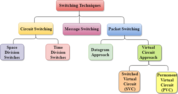
Classification Of Switching Techniques

---

Circuit Switching

• Circuit switching is a switching technique that establishes a dedicated path between sender and receiver.
• In the Circuit Switching Technique, once the connection is established then the dedicated path will remain to exist until the connection is terminated.
• Circuit switching in a network operates in a similar way as the telephone works.
• A complete end-to-end path must exist before the communication takes place.
• In case of circuit switching technique, when any user wants to send the data, voice, video, a request signal is sent to the receiver then the receiver sends back the acknowledgment to ensure the availability of the dedicated path. After receiving the acknowledgment, dedicated path transfers the data.
• Circuit switching is used in public telephone network. It is used for voice transmission.
• Fixed data can be transferred at a time in circuit switching technology.

Communication through circuit switching has 3 phases:

• Circuit establishment
• Data transfer
• Circuit Disconnect

Circuit Switching can use either of the two technologies:

Space Division Switches:

• Space Division Switching is a circuit switching technology in which a single transmission path is accomplished in a switch by using a physically separate set of crosspoints.
• Space Division Switching can be achieved by using crossbar switch. A crossbar switch is a metallic crosspoint or semiconductor gate that can be enabled or disabled by a control unit.
• The Crossbar switch is made by using the semiconductor. For example, Xilinx crossbar switch using FPGAs.
• Space Division Switching has high speed, high capacity, and nonblocking switches.

Space Division Switches can be categorized in two ways:

• Crossbar Switch
• Multistage Switch

Crossbar Switch

The Crossbar switch is a switch that has n input lines and n output lines. The crossbar switch has n² intersection points known as crosspoints.

Disadvantage of Crossbar switch:

The number of crosspoints increases as the number of stations is increased. Therefore, it becomes very expensive for a large switch. The solution to this is to use a multistage switch.

Multistage Switch

• Multistage Switch is made by splitting the crossbar switch into the smaller units and then interconnecting them.
• It reduces the number of crosspoints.
• If one path fails, then there will be an availability of another path.

Advantages Of Circuit Switching:

• In the case of Circuit Switching technique, the communication channel is dedicated.
• It has fixed bandwidth.

Disadvantages Of Circuit Switching:

• Once the dedicated path is established, the only delay occurs in the speed of data transmission.
• It takes a long time to establish a connection approx 10 seconds during which no data can be transmitted.
• It is more expensive than other switching techniques as a dedicated path is required for each connection.
• It is inefficient to use because once the path is established and no data is transferred, then the capacity of the path is wasted.
• In this case, the connection is dedicated therefore no other data can be transferred even if the channel is free.

---

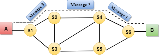
Message Switching

• Message Switching is a switching technique in which a message is transferred as a complete unit and routed through intermediate nodes at which it is stored and forwarded.
• In Message Switching technique, there is no establishment of a dedicated path between the sender and receiver.
• The destination address is appended to the message. Message Switching provides a dynamic routing as the message is routed through the intermediate nodes based on the information available in the message.
• Message switches are programmed in such a way so that they can provide the most efficient routes.
• Each and every node stores the entire message and then forward it to the next node. This type of network is known as store and forward network.
• Message switching treats each message as an independent entity.

Advantages Of Message Switching

• Data channels are shared among the communicating devices that improve the efficiency of using available bandwidth.
• Traffic congestion can be reduced because the message is temporarily stored in the nodes.
• Message priority can be used to manage the network.
• The size of the message which is sent over the network can be varied. Therefore, it supports the data of unlimited size.

Disadvantages Of Message Switching

• The message switches must be equipped with sufficient storage to enable them to store the messages until the message is forwarded.
• The Long delay can occur due to the storing and forwarding facility provided by the message switching technique.

---

Packet Switching

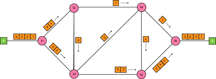
• The packet switching is a switching technique in which the message is sent in one go, but it is divided into smaller pieces, and they are sent individually.
• The message splits into smaller pieces known as packets and packets are given a unique number to identify their order at the receiving end.
• Every packet contains some information in its headers such as source address, destination address and sequence number.
• Packets will travel across the network, taking the shortest path as possible.
• All the packets are reassembled at the receiving end in correct order.
• If any packet is missing or corrupted, then the message will be sent to resend the message.
• If the correct order of the packets is reached, then the acknowledgment message will be sent.

Approaches Of Packet Switching:

There are two approaches to Packet Switching:

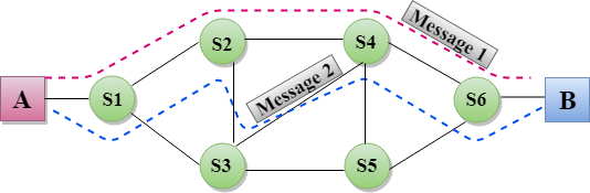
Datagram Packet switching:

• It is a packet switching technology in which packet is known as a datagram, is considered as an independent entity. Each packet contains the information about the destination and switch uses this information to forward the packet to the correct destination.
• The packets are reassembled at the receiving end in correct order.
• In Datagram Packet Switching technique, the path is not fixed.
• Intermediate nodes take the routing decisions to forward the packets.
• Datagram Packet Switching is also known as connectionless switching.

Virtual Circuit Switching

• Virtual Circuit Switching is also known as connection-oriented switching.
• In the case of Virtual circuit switching, a preplanned route is established before the messages are sent.
• Call request and call accept packets are used to establish the connection between sender and receiver.
• In this case, the path is fixed for the duration of a logical connection.

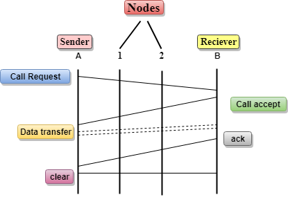
Let's understand the concept of virtual circuit switching through a diagram:

• In the above diagram, A and B are the sender and receiver respectively. 1 and 2 are the nodes.
• Call request and call accept packets are used to establish a connection between the sender and receiver.
• When a route is established, data will be transferred.
• After transmission of data, an acknowledgment signal is sent by the receiver that the message has been received.
• If the user wants to terminate the connection, a clear signal is sent for the termination.

---

Differences b/w Datagram approach and Virtual Circuit approach

Datagram approach	Virtual Circuit approach
Node takes routing decisions to forward the packets.	Node does not take any routing decision.
Congestion cannot occur as all the packets travel in different directions.	Congestion can occur when the node is busy, and it does not allow other packets to pass through.
It is more flexible as all the packets are treated as an independent entity.	It is not very flexible.

Cost-effective: In packet switching technique, switching devices do not require massive secondary storage to store the packets, so cost is minimized to some extent. Therefore, we can say that the packet switching technique is a cost-effective technique.Advantages Of Packet Switching:

• Reliable: If any node is busy, then the packets can be rerouted. This ensures that the Packet Switching technique provides reliable communication.
• Efficient: Packet Switching is an efficient technique. It does not require any established path prior to the transmission, and many users can use the same communication channel simultaneously, hence makes use of available bandwidth very efficiently.

Disadvantages Of Packet Switching:

• Packet Switching technique cannot be implemented in those applications that require low delay and high-quality services.
• The protocols used in a packet switching technique are very complex and requires high implementation cost.
• If the network is overloaded or corrupted, then it requires retransmission of lost packets. It can also lead to the loss of critical information if errors are nor recovered.

Transmission Impairments

In the data communication system, analog and digital signals go through the transmission medium. Transmission media are not ideal. There are some imperfections in transmission mediums. So, the signals sent through the transmission medium are also not perfect. This imperfection cause signal impairment.

It means that signals that are transmitted at the beginning of the medium are not the same as the signals that are received at the end of the medium that is what is sent is not what is received. These impairments tend to deteriorate the quality of analog and digital signals.

Consequences

1. For a digital signal, there may occur bit errors.
2. For analog signals, these impairments degrade the quality of the signals.

Causes of impairment

There are three main causes of impairment are,

1. Attenuation
2. Distortion
3. Noise

1) Attenuation

Here attenuation Means loss of energy that is the weaker signal. Whenever a signal transmitted through a medium it loses its energy, so that it can overcome by the resistance of the medium.

• That is why a wire carrying electrical signals gets warm, if not hot, after a while. Some of the electrical energy is converted to heat in the signal.
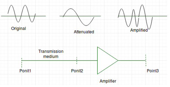
• Amplifiers are used to amplify the signals to compensate for this loss.
• This figure shows the effect of attenuation and amplification:





• A signal has lost or gained its strength, for this purpose engineers use the concept of decibel(dB).
• Decibel is used to measure the relative strengths of two signals or a signal at two different points.
• If a signal is attenuated then dB is negative and if a signal is amplified so the db is positive.
  Attenuation(dB) = 10log10(P2/P1)
  where P2 and P1 are the power of a signal at points1 and 2.

2) Distortion

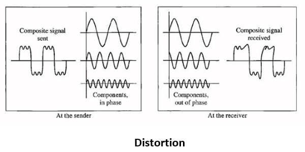
If a signal changes its form or shape, it is referred to as distortion. Signals made up of different frequencies are composite signals. Distortion occurs in these composite signals.

• Each component of frequency has its propagation speed traveling through a medium and therefore, different components have different delay in arriving at the final destination.
• It means that signals have different phases at the receiver than they did at the source.
• This figure shows the effect of distortion on a composite signal:

3) Noise

Noise is another problem. There are some random or unwanted signals mix up with the original signal is called noise. Noises can corrupt the signals in many ways along with the distortion introduced by the transmission media.

Different types of noises are:

1. Thermal noise
2. Intermodulation noise
3. Crosstalk
4. Impulse noise

a) Thermal noise

The thermal noise is random motion of electrons in a conductor that creates an extra signal not originally sent by the transmitter.

It is also known as white noise because it is distributed across the entire spectrum (as the frequency encompass over a broad range of frequencies).

b) Intermodulation noise

More than one signal share a single transmission channel, intermodulation noise is generated.

For instance, two signals S1 and S2 will generate signals of frequencies (S1 + S2) and (s1 - S2), which may interfere with the signals of the same frequencies sent by the sender. due to If nonlinearity present in any part of the communication system, intermodulation noise is introduced.

c) Cross talk

Cross talk is an effect a wire on the another. One wire acts as a sending antenna and the transmission medium acts as the receiving antenna.

Just like in telephone system, it is a common experience to hear conversation of other people in the background. This is known as cross talk.

d) Impulse noise

Impulse noise is irregular pulses or spikes( a signal with high energy in a very short period) generated by phenomena like that comes from power lines, lightning, spark due to loose contact in electric circuits and so on.

It is a primary source of bit-errors in digital data communication that kind of noise introduces burst errors.

Network Performance

Performance of a network pertains to the measure of service quality of a network as perceived by the user. There are different ways to measure the performance of a network, depending upon the nature and design of the network. The characteristics that measure the performance of a network are :

• Bandwidth
• Throughput
• Latency (Delay)
• Bandwidth – Delay Product
• Jitter

BANDWIDTH

One of the most essential conditions of a website’s performance is the amount of bandwidth allocated to the network. Bandwidth determines how rapidly the web server is able to upload the requested information. While there are different factors to consider with respect to a site’s performance, bandwidth is every now and again the restricting element.

Bandwidth is characterized as the measure of data or information that can be transmitted in a fixed measure of time. The term can be used in two different contexts with two distinctive estimating values. In the case of digital devices, the bandwidth is measured in bits per second(bps) or bytes per second. In the case of analog devices, the bandwidth is measured in cycles per second, or Hertz (Hz).

Bandwidth is only one component of what an individual sees as the speed of a network. People frequently mistake bandwidth with internet speed in light of the fact that internet service providers (ISPs) tend to claim that they have a fast “40Mbps connection” in their advertising campaigns. True internet speed is actually the amount of data you receive every second and that has a lot to do with latency too.

“Bandwidth” means “Capacity” and “Speed” means “Transfer rate”.

More bandwidth does not mean more speed. Let us take a case where we have double the width of the tap pipe, but the water rate is still the same as it was when the tap pipe was half the width. Hence, there will be no improvement in speed. When we consider WAN links, we mostly mean bandwidth but when we consider LAN, we mostly mean speed. This is on the grounds that we are generally constrained by expensive cable bandwidth over WAN rather than hardware and interface data transfer rates (or speed) over LAN.

Bandwidth in Hertz : It is the range of frequencies contained in a composite signal or the range of frequencies a channel can pass. For example, let us consider the bandwidth of a subscriber telephone line as 4 kHz.

Bandwidth in Bits per Seconds : It refers to the number of bits per second that a channel, a link, or rather a network can transmit. For example, we can say the bandwidth of a fast Ethernet network is a maximum of 100 Mbps, which means that the network can send 100 Mbps of data.

Note: There exists an explicit relationship between the bandwidth in hertz and the bandwidth in bits per second. An increase in bandwidth in hertz means an increase in bandwidth in bits per seconds. The relationship depends upon whether we have baseband transmission or transmission with modulation.

THROUGHPUT

Throughput is the number of messages successfully transmitted per unit time. It is controlled by available bandwidth, the available signal-to-noise ratio and the hardware limitations. The maximum throughput of a network may be consequently higher than the actual throughput achieved in everyday consumption. The terms ‘throughput’ and ‘bandwidth’ are often thought of as the same, yet they are different. Bandwidth is the potential measurement of a link, whereas throughput is an actual measurement of how fast we can send data.

Throughput is measured by tabulating the amount of data transferred between multiple locations during a specific period of time, usually resulting in the unit of bits per second(bps), which has evolved to bytes per second(Bps), kilobytes per second(KBps), megabytes per second(MBps) and gigabytes per second(GBps). Throughput may be affected by numerous factors, such as the hindrance of the underlying analog physical medium, available processing power of the system components, and end-user behavior. When numerous protocol expenses are taken into account, the useful rate of the transferred data can be significantly lower than the maximum achievable throughput.

Let us consider: A highway which has a capacity of moving, say, 200 vehicles at a time. But at a random time someone notices only, say, 150 vehicles moving through it due to some congestion on the road. As a result, the capacity is likely to be 200 vehicles per unit time and the throughput is 150 vehicles at a time.

Example:

Input:A network with bandwidth of 10 Mbps can pass only an average of 12, 000 frames 
per minute where each frame carries an average of 10, 000 bits. What will be the 
throughput for this network?

Output: We can calculate the throughput as-
Throughput = (12, 000 x 10, 000) / 60 = 2 Mbps
The throughput is nearly equal to one-fifth of the bandwidth in this case.

LATENCY

In a network, during the process of data communication, latency(also known as delay) is defined as the total time taken for a complete message to arrive at the destination, starting with the time when the first bit of the message is sent out from the source and ending with the time when the last bit of the message is delivered at the destination. The network connections where small delays occur are called “Low-Latency-Networks” and the network connections which suffer from long delays are known as “High-Latency-Networks”.

High latency leads to creation of bottlenecks in any network communication. It stops the data from taking full advantage of the network pipe and conclusively decreases the bandwidth of the communicating network. The effect of the latency on a network’s bandwidth can be temporary or never-ending depending on the source of the delays. Latency is also known as a ping rate and measured in milliseconds(ms).

In simpler terms: latency may be defined as the time required to successfully send a packet across a network.

It measured in many ways like: round trip, one way, etc.

It might be affected by any component in the chain which is utilized to vehiculate data, like: workstation, WAN links, routers, LAN, server and eventually may be limited for large networks, by the speed of light.

Latency = Propagation Time + Transmission Time + Queuing Time + Processing Delay

Propagation Time: It is the time required for a bit to travel from the source to the destination. Propagation time can be calculated as the ratio between the link length (distance) and the propagation speed over the communicating medium. For example, for an electric signal, propagation time is the time taken for the signal to travel through a wire.

Propagation time = Distance / Propagation speed

Example:

Input: What will be the propagation time when the distance between two points is
12, 000 km? Assuming the propagation speed to be 2.4 * 10^8 m/s in cable.

Output: We can calculate the propagation time as-
Propagation time = (12000 * 10000) / (2.4 * 10^8) = 50 ms 

Transmission Time: Transmission time is a time based on how long it takes to send the signal down the transmission line. It consists of time costs for an EM signal to propagate from one side to the other, or costs like the training signals that are usually put on the front of a packet by the sender, which helps the receiver synchronize clocks. The transmission time of a message relies upon the size of the message and bandwidth of the channel.

Transmission time = Message size / Bandwidth

Example:

Input:What will be the propagation time and the transmission time for a 2.5-kbyte 
message when the bandwidth of the network is 1 Gbps? Assuming the distance between
sender and receiver is 12, 000 km and speed of light is 2.4 * 10^8 m/s.

Output: We can calculate the propagation and transmission time as-
Propagation time = (12000 * 10000) / (2.4 * 10^8) = 50 ms
Transmission time = (2560 * 8) / 10^9 = 0.020 ms

Note: Since the message is short and the bandwidth is high, the dominant factor is the
propagation time and not the transmission time(which can be ignored).

Queuing Time: Queuing time is a time based on how long the packet has to sit around in the router. Quite frequently the wire is busy, so we are not able to transmit a packet immediately. The queuing time is usually not a fixed factor, hence it changes with the load thrust in the network. In cases like these, the packet sits waiting, ready to go, in a queue. These delays are predominantly characterized by the measure of traffic on the system. The more the traffic, the more likely a packet is stuck in the queue, just sitting in the memory, waiting.

Processing Delay: Processing delay is the delay based on how long it takes the router to figure out where to send the packet. As soon as the router finds it out, it will queue the packet for transmission. These costs are predominantly based on the complexity of the protocol. The router must decipher enough of the packet to make sense of which queue to put the packet in. Typically the lower level layers of the stack have simpler protocols. If a router does not know which physical port to send the packet to, it will send it to all the ports, queuing the packet in many queues immediately. Differently, at a higher level, like in IP protocols, the processing may include making an ARP request to find out the physical address of the destination before queuing the packet for transmission. This situation may also be considered as a processing delay.

BANDWIDTH – DELAY PRODUCT

Bandwidth and delay are two performance measurements of a link. However, what is significant in data communications is the product of the two, the bandwidth-delay product.

Let us take two hypothetical cases as examples.

Case 1: Assume a link is of bandwidth 1bps and the delay of the link is 5s. Let us find the bandwidth-delay product in this case. From the image, we can say that this product 1 x 5 is the maximum number of bits that can fill the link. There can be close to 5 bits at any time on the link.

Case 2: Assume a link is of bandwidth 3bps. From the image, we can say that there can be a maximum 3 x 5 = 15 bits on the line. The reason is that, at each second, there are 3 bits on the line and the duration of each bit is 0.33s.

For both the examples, the product of bandwidth and delay is the number of bits that can fill the link. This estimation is significant in the event that we have to send data in bursts and wait for the acknowledgment of each burst before sending the following one. To utilize the maximum ability of the link, we have to make the size of our burst twice the product of bandwidth and delay. Also, we need to fill up the full-duplex channel. The sender ought send a burst of data of (2*bandwidth*delay) bits. The sender at that point waits for the receiver’s acknowledgment for part of the burst before sending another burst. The amount: 2*bandwidth*delay is the number of bits that can be in transition at any time.

JITTER

Jitter is another performance issue related to delay. In technical terms, jitter is a “packet delay variance”. It can simply mean that jitter is considered as a problem when different packets of data face different delays in a network and the data at the receiver application is time-sensitive, i.e. audio or video data. Jitter is measured in milliseconds(ms). It is defined as an interference in the normal order of sending data packets. For example: if the delay for the first packet is 10 ms, for the second is 35 ms, and for the third is 50 ms, then the real-time destination application that uses the packets experiences jitter.

Simply, jitter is any deviation in, or displacement of, the signal pulses in a high-frequency digital signal. The deviation can be in connection with the amplitude, the width of the signal pulse or the phase timing. The major causes of jitter are: electromagnetic interference(EMI) and crosstalk between signals. Jitter can lead to flickering of a display screen, affects in the capability of a processor in a desktop or server to proceed as expected, introducing clicks or other undesired impacts in audio signals, and loss of transmitted data between network devices.

Jitter is negative and causes network congestion and packet loss.

Congestion is like a traffic jam on the highway. In a traffic jam, cars cannot move forward at a reasonable speed. Like the traffic jam, in congestion all the packets come to a junction at the same time. Nothing can get loaded.

The second negative effect is packet loss. When packets arrive at unexpected intervals, the receiving system is not able to process the information, which leads to missing information also called “packet loss”. This has negative effects for video viewing. If a video becomes pixelated and is skipping, the network is experiencing jitter. The result of the jitter is packet loss. When you are playing a game online, the effect of packet loss can be that a player begins moving around on the screen randomly. Even worse, the game goes from one scene to the next, skipping over part of the game play.

In the above image, it can be noticed that the time it takes for packets to be sent is not the same as the time in which he will arrive at the receiver side. One of the packets faces an unexpected delay on its way and is received after the expected time. This is jitter.

A jitter buffer can reduce the effects of jitter, either in a network, on a router or switch, or on a computer. The system at the destination receiving the network packets usually receive them from the buffer and not from the source system directly. Each packet is fed out of the buffer at a regular rate. Another approach to diminish jitter in case of multiple paths for traffic is to selectively route traffic along the most stable paths, or to always pick the path that can come closest to the targeted packet delivery rate.