Branch and bound
Branch & bound is a well-known technique that is mainly used to solve problems categorized as optimization problems
It is an improvement over an exhaustive search because B&B builds applicant solutions one part at a time and assesses the built arrangements as unmistakable parts.
B & B is based on a state space tree. The state space tree is the root of the tree where every level represents a decision in the solution space that relies on the upper level and any conceivable solution is represented in a few ways beginning at the root and finishing with a leaf. It is an enhancement of backtracking
Difference
BackTracking | Branch & Bound |
| It follows depth depth-first search approach | It follows breadth-first search approach |
| It takes comparatively more time for execution. | It takes less time for execution. |
| Used to find all possible solutions available to the problem. | It is used to solve optimization problems. |
- The branch-and-bound algorithm does not limit us to any particular way of traversing the tree.
- Used only for optimization problems (since the backtracking algorithm requires the use of DFS traversal and is used for non-optimization problems.
Theory
A branch and bound algorithm consists of a systematic enumeration of candidate solutions by means of state space search: the set of candidate solutions is thought of as forming a rooted tree with the full set at the root.
- It is a systematic method for solving optimization problems
- B&B is a rather general optimization technique that applies where the greedy method and dynamic programming fail.
- However, it is much slower. Indeed, it often leads to exponential time complexities in the worst case.
- On the other hand, if applied carefully, it can lead to algorithms that run reasonably fast on average.
Applications
- Nonlinear programming
- Travelling salesman problem (TSP)
- Maximum satisfiability problem (MAX-SAT)
- Nearest neighbor search
- Parameter estimation
- 0/1 knapsack problem
- Feature selection in machine learning
Let's understand through an example.
Jobs = {j1, j2, j3, j4}
P = {10, 5, 8, 3}
d = {1, 2, 1, 2}
The above are jobs, problems and problems given. We can write the solutions in two ways which are given below:
Suppose we want to perform the jobs j1 and j2 then the solution can be represented in two ways:
The first way of representing the solutions is the subsets of jobs.
S1 = {j1, j4}
The second way of representing the solution is that first job is done, second and third jobs are not done, and fourth job is done.
S2 = {1, 0, 0, 1}
The solution s1 is the variable-size solution while the solution s2 is the fixed-size solution.
First, we will see the subset method where we will see the variable size.
First method:
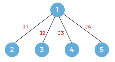
In this case, we first consider the first job, then second job, then third job and finally we consider the last job.
As we can observe in the above figure that the breadth first search is performed but not the depth first search. Here we move breadth wise for exploring the solutions. In backtracking, we go depth-wise whereas in branch and bound, we go breadth wise.
Now one level is completed. Once I take first job, then we can consider either j2, j3 or j4. If we follow the route then it says that we are doing jobs j1 and j4 so we will not consider jobs j2 and j3.
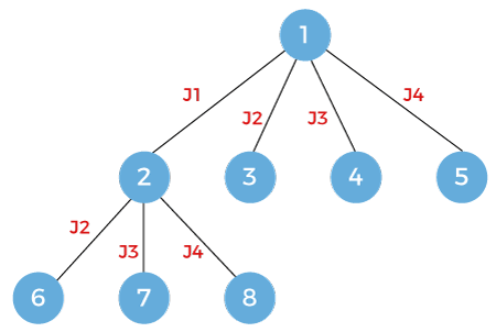
Now we will consider the node 3. In this case, we are doing job j2 so we can consider either job j3 or j4. Here, we have discarded the job j1.
Now we will expand the node 4. Since here we are doing job j3 so we will consider only job j4.
Now we will expand node 6, and here we will consider the jobs j3 and j4.
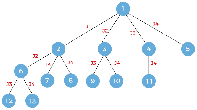
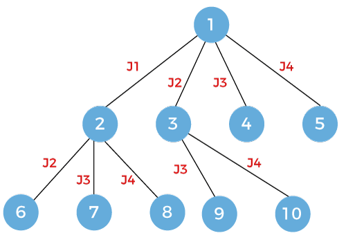
Now we will expand node 7 and here we will consider job j4.
Now we will expand node 9, and here we will consider job j4.
The last node, i.e., node 12 which is left to be expanded. Here, we consider job j4.
The above is the state space tree for the solution s1 = {j1, j4}
Second method:
We will see another way to solve the problem to achieve the solution s1.
First, we consider the node 1 shown as below:
Now, we will expand the node 1. After expansion, the state space tree would be appeared as:
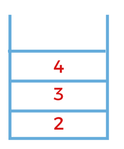
On each expansion, the node will be pushed into the stack shown as below:
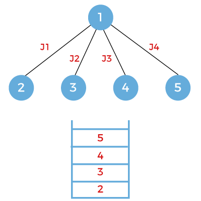
Now the expansion would be based on the node that appears on the top of the stack. Since the node 5 appears on the top of the stack, so we will expand the node 5. We will pop out the node 5 from the stack. Since the node 5 is in the last job, i.e., j4 so there is no further scope of expansion.
The next node that appears on the top of the stack is node 4. Pop out the node 4 and expand. On expansion, job j4 will be considered and node 6 will be added into the stack shown as below:
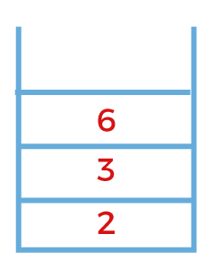
The next node is 6 which is to be expanded. Pop out the node 6 and expand. Since the node 6 is in the last job, i.e., j4 so there is no further scope of expansion.
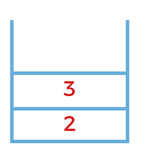
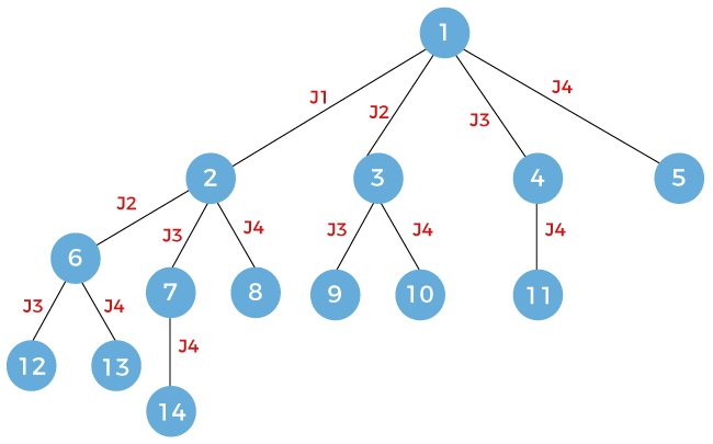
The next node to be expanded is node 3. Since the node 3 works on the job j2 so node 3 will be expanded to two nodes, i.e., 7 and 8 working on jobs 3 and 4 respectively. The nodes 7 and 8 will be pushed into the stack shown as below:
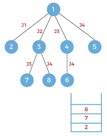
The next node that appears on the top of the stack is node 8. Pop out the node 8 and expand. Since the node 8 works on the job j4 so there is no further scope for the expansion.
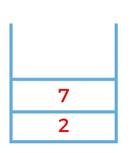
The next node that appears on the top of the stack is node 7. Pop out the node 7 and expand. Since the node 7 works on the job j3 so node 7 will be further expanded to node 9 that works on the job j4 as shown as below and the node 9 will be pushed into the stack.
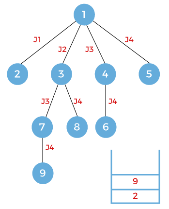
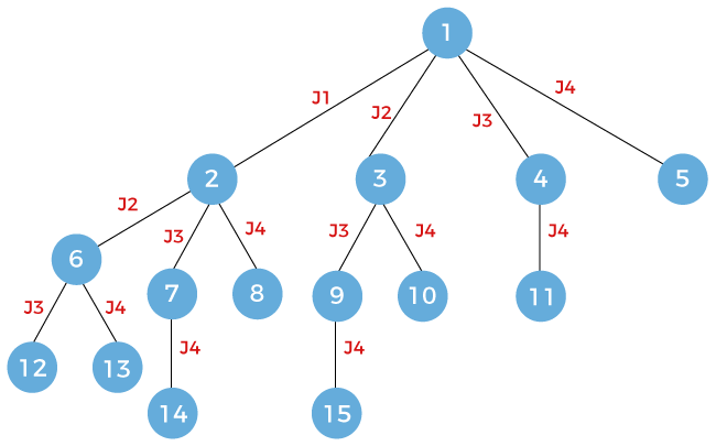
The next node that appears on the top of the stack is node 9. Since the node 9 works on the job 4 so there is no further scope for the expansion.
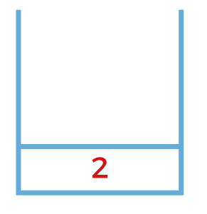
The next node that appears on the top of the stack is node 2. Since the node 2 works on the job j1 so it means that the node 2 can be further expanded. It can be expanded upto three nodes named as 10, 11, 12 working on jobs j2, j3, and j4 respectively. There newly nodes will be pushed into the stack shown as below:
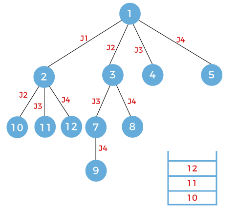
In the above method, we explored all the nodes using the stack that follows the LIFO principle.
Third method
There is one more method that can be used to find the solution and that method is Least cost branch and bound. In this technique, nodes are explored based on the cost of the node. The cost of the node can be defined using the problem and with the help of the given problem, we can define the cost function. Once the cost function is defined, we can define the cost of the node.
Let's first consider the node 1 having cost infinity shown as below:
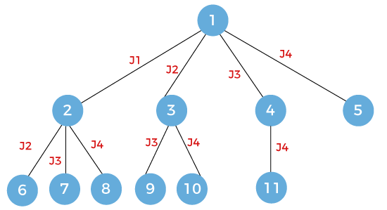
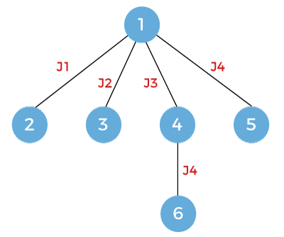
Now we will expand the node 1. The node 1 will be expanded into four nodes named as 2, 3, 4 and 5 shown as below:
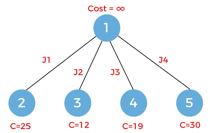
Let's assume that cost of the nodes 2, 3, 4, and 5 are 25, 12, 19 and 30 respectively.
Since it is the least cost branch n bound, so we will explore the node which is having the least cost. In the above figure, we can observe that the node with a minimum cost is node 3. So, we will explore the node 3 having cost 12.
Since the node 3 works on the job j2 so it will be expanded into two nodes named as 6 and 7 shown as below:
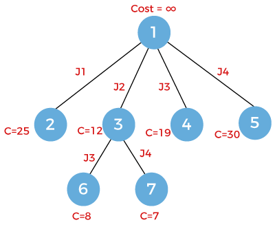
The node 6 works on job j3 while the node 7 works on job j4. The cost of the node 6 is 8 and the cost of the node 7 is 7. Now we have to select the node which is having the minimum cost. The node 7 has the minimum cost so we will explore the node 7. Since the node 7 already works on the job j4 so there is no further scope for the expansion.


No comments:
Post a Comment