K-Nearest Neighbor(KNN) Algorithm 

• K-Nearest Neighbour is one of the simplest Machine Learning algorithms based on Supervised Learning technique.
• K-NN algorithm assumes the similarity between the new case/data and available cases and put the new case into the category that is most similar to the available categories.
• K-NN algorithm stores all the available data and classifies a new data point based on the similarity. This means when new data appears then it can be easily classified into a well suite category by using K- NN algorithm.
• K-NN algorithm can be used for Regression as well as for Classification but mostly it is used for the Classification problems.
• K-NN is a non-parametric algorithm, which means it does not make any assumption on underlying data.
• It is also called a lazy learner algorithm because it does not learn from the training set immediately instead it stores the dataset and at the time of classification, it performs an action on the dataset.
• KNN algorithm at the training phase just stores the dataset and when it gets new data, then it classifies that data into a category that is much similar to the new data.
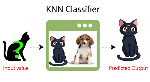
• Example: Suppose, we have an image of a creature that looks similar to cat and dog, but we want to know either it is a cat or dog. So for this identification, we can use the KNN algorithm, as it works on a similarity measure. Our KNN model will find the similar features of the new data set to the cats and dogs images and based on the most similar features it will put it in either cat or dog category.

Why do we need a K-NN Algorithm?

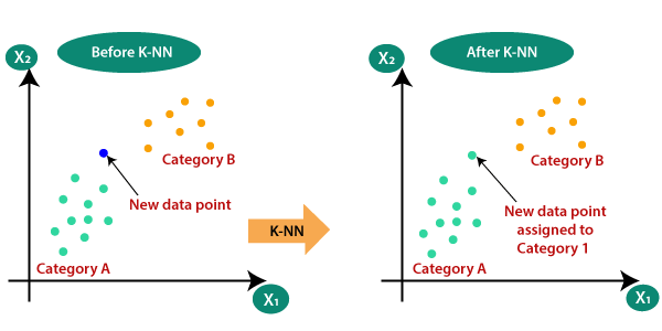
Suppose there are two categories, i.e., Category A and Category B, and we have a new data point x1, so this data point will lie in which of these categories. To solve this type of problem, we need a K-NN algorithm. With the help of K-NN, we can easily identify the category or class of a particular dataset. Consider the below diagram:

How does K-NN work?

The K-NN working can be explained on the basis of the below algorithm:

• Step-1: Select the number K of the neighbors
• Step-2: Calculate the Euclidean distance of K number of neighbors
• Step-3: Take the K nearest neighbors as per the calculated Euclidean distance.
• Step-4: Among these k neighbors, count the number of the data points in each category.
• Step-5: Assign the new data points to that category for which the number of the neighbor is maximum.
• Step-6: Our model is ready.

Suppose we have a new data point and we need to put it in the required category. Consider the below image:

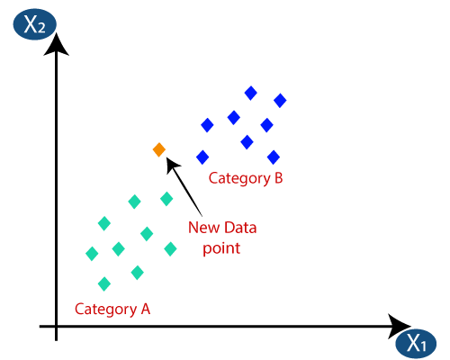
• Firstly, we will choose the number of neighbors, so we will choose the k=5.
• Next, we will calculate the Euclidean distance between the data points. The Euclidean distance is the distance between two points, which we have already studied in geometry. It can be calculated as:

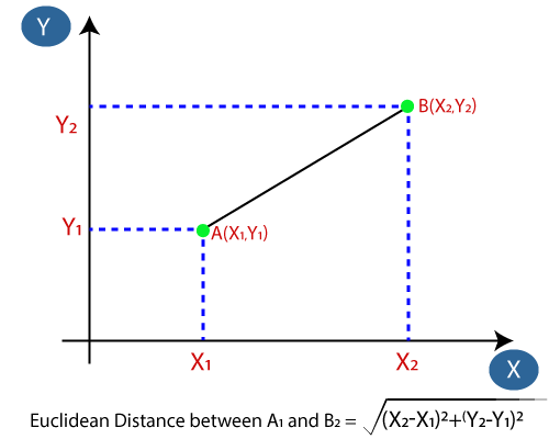
• By calculating the Euclidean distance we got the nearest neighbors, as three nearest neighbors in category A and two nearest neighbors in category B. Consider the below image:

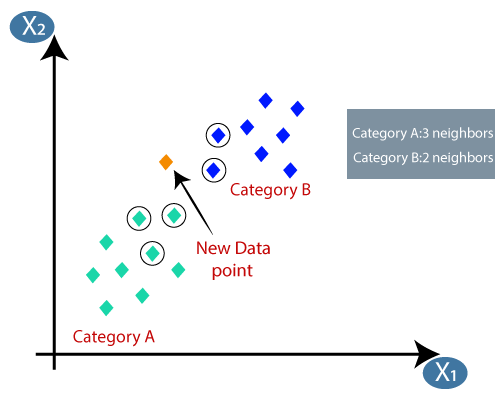
• As we can see the 3 nearest neighbors are from category A, hence this new data point must belong to category A.

How to select the value of K in the K-NN Algorithm?

Below are some points to remember while selecting the value of K in the K-NN algorithm:

• There is no particular way to determine the best value for "K", so we need to try some values to find the best out of them. The most preferred value for K is 5.
• A very low value for K such as K=1 or K=2, can be noisy and lead to the effects of outliers in the model.
• Large values for K are good, but it may find some difficulties.

Advantages of KNN Algorithm:

• It is simple to implement.
• It is robust to the noisy training data
• It can be more effective if the training data is large.

Disadvantages of KNN Algorithm:

• Always needs to determine the value of K which may be complex some time.
• The computation cost is high because of calculating the distance between the data points for all the training samples.

Example

We have data from the questionnaires survey (to ask people opinion) and objective testing with two attributes (acid durability and strength) to classify whether a special paper tissue is good or not. Here is four training samples

X1 = Acid Durability (seconds)	X2 = Strength (kg/square meter)	Y = Classification
7	7	Bad
7	4	Bad
3	4	Good
1	4	Good

Now the factory produces a new paper tissue that pass laboratory test with X1 = 3 and X2 = 7. Without another expensive survey, can we guess what the classification of this new tissue is?

1. Determine parameter K = number of nearest neighbors

Suppose use K = 3

2. Calculate the distance between the query-instance and all the training samples

Coordinate of query instance is (3, 7), instead of calculating the distance we compute square distance which is faster to calculate (without square root)

X1 = Acid Durability (seconds)	X2 = Strength (kg/square meter)	Square Distance to query instance (3, 7)
7	7
7	4
3	4
1	4

3. Sort the distance and determine nearest neighbors based on the K-th minimum distance

X1 = Acid Durability (seconds)	X2 = Strength (kg/square meter)	Square Distance to query instance (3, 7)	Rank minimum distance	Is it included in 3-Nearest neighbors?
7	7		3	Yes
7	4		4	No
3	4		1	Yes
1	4		2	Yes

4. Gather the category  of the nearest neighbors. Notice in the second row last column that the category of nearest neighbor (Y) is not included because the rank of this data is more than 3 (=K).

X1 = Acid Durability (seconds)	X2 = Strength (kg/square meter)	Square Distance to query instance (3, 7)	Rank minimum distance	Is it included in 3-Nearest neighbors?	Y = Category of nearest Neighbor
7	7		3	Yes	Bad
7	4		4	No	-
3	4		1	Yes	Good
1	4		2	Yes	Good

5. Use simple majority of the category of nearest neighbors as the prediction value of the query instance

We have 2 good and 1 bad, since 2>1 then we conclude that a new paper tissue that pass laboratory test with X1 = 3 and X2 = 7 is included in Good category.

Example: Consider a dataset that contains two variables: height (cm) & weight (kg). Each point is classified as normal or underweight.

Based on the above data, you need to classify the following set as normal or underweight using the KNN algorithm.

To find the nearest neighbors, we will calculate the Euclidean distance.

The Euclidean distance between two points in the plane with coordinates (x,y) and (a,b) is given by:

Let us calculate the Euclidean distance with the help of unknown data points.

The following table shows the calculated Euclidean distance of unknown data points from all points.

Now, we have a new data point (x1, y1), and we need to determine its class. 

Looking at the new data, we can consider the last three rows from the table—K=3.

Since the majority of neighbors are classified as normal as per the KNN algorithm, the data point (57, 170) should be normal.

Ques. Describe K-nearest neighbour algorithm with steps.

Answer:

K-Nearest-neighbour classifier 

Uses k “closest” points (nearest neighbours) for performing classification.

K-Nearest Neighbor algorithms classify a new example by comparing it to all previously seen examples. 

The classifications of the k most similar previous cases are used for predicting the classification of the current example.

Algo: 

1. Compare new example, x, to each case, y, in the case base and calculate for each pair:

where match(a, b) is a function that returns 1 if a and b are equal and 0 otherwise.

2. Let R = the top k cases ranked according to sim 

3. Return as f(x) the class, c, that wins the majority vote among f(R1), f(R2),...,f(R|k|). Handle ties randomly.

 

Ques. What are the advantages and disadvantages of K-nearest neighbour algorithm?

Answer:

Advantages of K-nearest neighbour:

1. No Training Period
2. Since the KNN algorithm requires no training before making predictions, new data can be added seamlessly which will not impact the accuracy of the algorithm.
3. KNN is very easy to implement. 

Disadvantages of K-nearest neighbour:

1. Does not work well with large dataset
2. Does not work well with high dimensions
3. Need feature scaling
4. Sensitive to noisy data, missing values and outliers

Ques. Explain locally weighted regression.

Answer:

Locally weighted regression (LWR) is a memory-based method that performs a regression around a point of interest using only training data that are ``local'' to that point.

• It allows to adjust the regression models to nearby data.
• It allows to improve the overall performance of regression methods by adjusting the capacity of the models to the properties of the training data in each area of the input space 
• Examples of locally weighted learning methods include k-Nearest Neighbours (kNN) and Locally Weighted Regression methods.

Applications:

• Numerical Analysis
• Sociology
• Economics
• Chemometrics 
• Computer Graphics
• Robot Learning and Control 

Ques. Explain Radial Basis Function(RBF).

Answer:

1. The most used type of kernel function is Radial Based Function.
2. Because it has localized and finite response along the entire x-axis.
3. It is a general-purpose kernel; used when there is no prior knowledge about the data.
   Equation is:

for:

1. ||xi - xj||2 is the Euclidean Distance between xi and xj.
2. RBF kernel is a function whose value depends on the distance from the origin or from some point.
3. Radial basis function networks are distinguished from other neural networks due to their universal approximation and faster learning speed. 
4. An RBF network is a type of feed forward neural network composed of three layers, namely the input layer, the hidden layer and the output layer.
5. Global approximation to target function, in terms of linear combination of local approximations 
6. Used in image classification 
7. It is a different kind of neural network 
8. Closely related to distance-weighted regression, but “eager” instead of “lazy

 

Ques. Explain the architecture of a radial basis function network.

Answer:

Architecture:

RBF network is an artificial neural network with an input layer, a hidden layer, and an output layer. The Hidden layer of RBF consists of hidden neurons, and the activation function of these neurons is a Gaussian function. Hidden layer generates a signal corresponding to an input vector in the input layer, and corresponding to this signal, the network generates a response.

In RBF architecture, weights connecting input vectors to hidden neurons represent the center of the corresponding neuron.