Case study of CNN for eg on Diabetic Retinopathy, Building a smart speaker, Self-deriving car etc.

Case Study of CNN for Diabetic retinopathy :

• Diabetic retinopathy also known as diabetic eye disease, is a medical state in which destruction occurs to the retina due to diabetes mellitus, It is a major cause of blindness in advance countries.
• Diabetic retinopathy influence up to 80 percent of those who have had diabetes for 20 years or more.
• The overlong a person has diabetes, the higher his or her chances of growing diabetic retinopathy.
• It is also the main cause of blindness in people of age group 20-64.
• Diabetic retinopathy is the outcome of destruction to the small blood vessels and neurons of the retina.

Case Study of CNN for Self-deriving car :

Convolutional neural networks (CNN) are used to model spatial information, such as images. CNNs are very good at extracting features from images, and they’re often seen as universal non-linear function approximators. 

CNNs can capture different patterns as the depth of the network increases. For example, the layers at the beginning of the network will capture edges, while the deep layers will capture more complex features like the shape of the objects (leaves in trees, or tires on a vehicle). This is the reason why CNNs are the main algorithm in self-driving cars. 

The key component of the CNN is the convolutional layer itself. It has a convolutional kernel which is often called the filter matrix. The filter matrix is convolved with a local region of the input image which can be defined as:

• Where: 
• 
  
• the operator * represents the convolution operation,

• w is the filter matrix and b is the bias, 

• x is the input,

• y is the output. 

The dimension of the filter matrix in practice is usually 3X3 or 5X5. During the training process, the filter matrix will constantly update itself to get a reasonable weight. One of the properties of CNN is that the weights are shareable. The same weight parameters can be used to represent two different transformations in the network. The shared parameter saves a lot of processing space; they can produce more diverse feature representations learned by the network.

• The output of the CNN is usually fed to a nonlinear activation function. The activation function enables the network to solve the linear inseparable problems, and these functions can represent high-dimensional manifolds in lower-dimensional manifolds. Commonly used activation functions are Sigmoid, Tanh, and ReLU, which are listed as follows:

It’s worth mentioning that the ReLU is the preferred activation function, because it converges faster compared to the other activation functions. In addition to that, the output of the convolution layer is modified by the max-pooling layer which keeps more information about the input image, like the background and texture. 

• The three important CNN properties that make them versatile and a primary component of self-driving cars are:

• local receptive fields, 
• shared weights, 
• spatial sampling. 

• These properties reduce overfitting and store representations and features that are vital for image classification, segmentation, localization, and more.

Case Study of CNN for Building a smart speaker :

Activation Function

What is Activation Function?

It’s just a thing function that you use to get the output of node. It is also known as Transfer Function.

Why we use Activation functions with Neural Networks?

It is used to determine the output of neural network like yes or no. It maps the resulting values in between 0 to 1 or -1 to 1 etc. (depending upon the function).

The Activation Functions can be basically divided into 2 types-

1.      Linear Activation Function

2.      Non-linear Activation Functions

Linear or Identity Activation Function

As you can see the function is a line or linear. Therefore, the output of the functions will not be confined between any range.

Fig: Linear Activation Function

Equation : f(x) = x

Range : (-infinity to infinity)

It doesn’t help with the complexity or various parameters of usual data that is fed to the neural networks.

Non-linear Activation Function

The Nonlinear Activation Functions are the most used activation functions. Nonlinearity helps to makes the graph look something like this

Fig: Non-linear Activation Function

It makes it easy for the model to generalize or adapt with variety of data and to differentiate between the output.

The main terminologies needed to understand for nonlinear functions are:

Derivative or Differential: Change in y-axis w.r.t. change in x-axis.It is also known as slope.

Monotonic function: A function which is either entirely non-increasing or non-decreasing.

The Nonlinear Activation Functions are mainly divided on the basis of their range or curves-

1. Sigmoid or Logistic Activation Function

The Sigmoid Function curve looks like a S-shape.

Fig: Sigmoid Function

The main reason why we use sigmoid function is because it exists between (0 to 1). Therefore, it is especially used for models where we have to predict the probability as an output.Since probability of anything exists only between the range of 0 and 1, sigmoid is the right choice.
The function is differentiable.That means, we can find the slope of the sigmoid curve at any two points.
The function is monotonic but function’s derivative is not.
The logistic sigmoid function can cause a neural network to get stuck at the training time.
The softmax function is a more generalized logistic activation function which is used for multiclass classification.

Convolutional Neural Network (CNN)

Convolutional Neural Network

Convolutional Neural Network is one of the main categories to do image classification and image recognition in neural networks. Scene labeling, objects detections, and face recognition, etc., are some of the areas where convolutional neural networks are widely used.

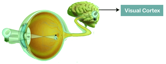
Convolutional Neural Networks are a special type of feed-forward artificial neural network in which the connectivity pattern between its neuron is inspired by the visual cortex.

The visual cortex encompasses a small region of cells that are region sensitive to visual fields. In case some certain orientation edges are present then only some individual neuronal cells get fired inside the brain such as some neurons responds as and when they get exposed to the vertical edges, however some responds when they are shown to horizontal or diagonal edges, which is nothing but the motivation behind Convolutional Neural Networks.

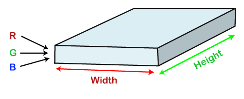
The Convolutional Neural Networks, which are also called as covnets, are nothing but neural networks, sharing their parameters. Suppose that there is an image, which is embodied as a cuboid, such that it encompasses length, width, and height. Here the dimensions of the image are represented by the Red, Green, and Blue channels, as shown in the image given below.

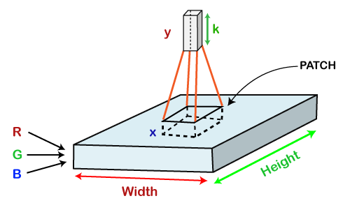
Now assume that we have taken a small patch of the same image, followed by running a small neural network on it, having k number of outputs, which is represented in a vertical manner. Now when we slide our small neural network all over the image, it will result in another image constituting different width, height as well as depth. We will notice that rather than having R, G, B channels, we have come across some more channels that, too, with less width and height, which is actually the concept of Convolution. In case, if we accomplished in having similar patch size as that of the image, then it would have been a regular neural network. We have some wights due to this small patch.

Mathematically it could be understood as follows;

• The Convolutional layers encompass a set of learnable filters, such that each filter embraces small width, height as well as depth as that of the provided input volume (if the image is the input layer then probably it would be 3).
• Suppose that we want to run the convolution over the image that comprises of 34x34x3 dimension, such that the size of a filter can be axax3. Here a can be any of the above 3, 5, 7, etc. It must be small in comparison to the dimension of the image.
• Each filter gets slide all over the input volume during the forward pass. It slides step by step, calling each individual step as a stride that encompasses a value of 2 or 3 or 4 for higher-dimensional images, followed by calculating a dot product in between filter's weights and patch from input volume.
• It will result in 2-Dimensional output for each filter as and when we slide our filters followed by stacking them together so as to achieve an output volume to have a similar depth value as that of the number of filters. And then, the network will learn all the filters.

Working of CNN

Generally, a Convolutional Neural Network has three layers, which are as follows;

• Input: If the image consists of 32 widths, 32 height encompassing three R, G, B channels, then it will hold the raw pixel([32x32x3]) values of an image.
• Convolution: It computes the output of those neurons, which are associated with input's local regions, such that each neuron will calculate a dot product in between weights and a small region to which they are actually linked to in the input volume. For example, if we choose to incorporate 12 filters, then it will result in a volume of [32x32x12].
• ReLU(Rectified Linear Activation Function) Layer: It is specially used to apply an activation function elementwise, like as max (0, x) thresholding at zero. It results in ([32x32x12]), which relates to an unchanged size of the volume.
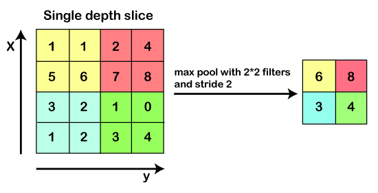
• Pooling: This layer is used to perform a downsampling operation along the spatial dimensions (width, height) that results in [16x16x12] volume.
  
• Locally Connected: It can be defined as a regular neural network layer that receives an input from the preceding layer followed by computing the class scores and results in a 1-Dimensional array that has the equal size to that of the number of classes.
  

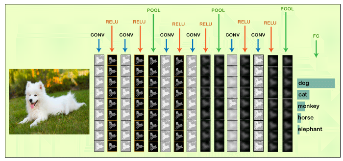
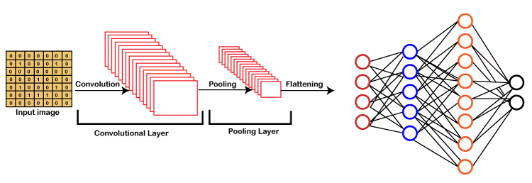
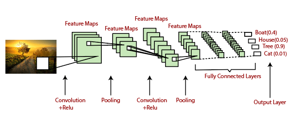
We will start with an input image to which we will be applying multiple feature detectors, which are also called as filters to create the feature maps that comprises of a Convolution layer. Then on the top of that layer, we will be applying the ReLU or Rectified Linear Unit to remove any linearity or increase non-linearity in our images.

Next, we will apply a Pooling layer to our Convolutional layer, so that from every feature map we create a Pooled feature map as the main purpose of the pooling layer is to make sure that we have spatial invariance in our images. It also helps to reduce the size of our images as well as avoid any kind of overfitting of our data. After that, we will flatten all of our pooled images into one long vector or column of all of these values, followed by inputting these values into our artificial neural network. Lastly, we will feed it into the locally connected layer to achieve the final output.

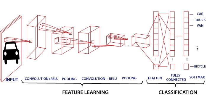
CNN takes an image as input, which is classified and process under a certain category such as dog, cat, lion, tiger, etc. The computer sees an image as an array of pixels and depends on the resolution of the image. Based on image resolution, it will see as h * w * d, where h= height w= width and d= dimension. For example, An RGB image is 6 * 6 * 3 array of the matrix, and the grayscale image is 4 * 4 * 1 array of the matrix.

In CNN, each input image will pass through a sequence of convolution layers along with pooling, fully connected layers, filters (Also known as kernels). After that, we will apply the Soft-max function to classify an object with probabilistic values 0 and 1.

Convolution Layer

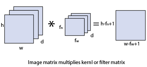
Convolution layer is the first layer to extract features from an input image. By learning image features using a small square of input data, the convolutional layer preserves the relationship between pixels. It is a mathematical operation which takes two inputs such as image matrix and a kernel or filter.

• The dimension of the image matrix is h×w×d.
• The dimension of the filter is f_h×f_w×d.
• The dimension of the output is (h-f_h+1)×(w-f_w+1)×1.

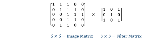
Let's start with consideration a 5*5 image whose pixel values are 0, 1, and filter matrix 3*3 as:

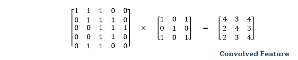
The convolution of 5*5 image matrix multiplies with 3*3 filter matrix is called "Features Map" and show as an output.

Convolution of an image with different filters can perform an operation such as blur, sharpen, and edge detection by applying filters.

Strides

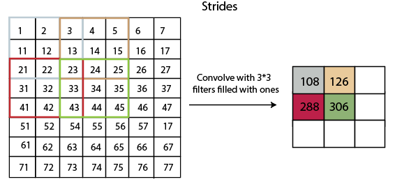
Stride is the number of pixels which are shift over the input matrix. When the stride is equaled to 1, then we move the filters to 1 pixel at a time and similarly, if the stride is equaled to 2, then we move the filters to 2 pixels at a time. The following figure shows that the convolution would work with a stride of 2.

Padding

Padding plays a crucial role in building the convolutional neural network. If the image will get shrink and if we will take a neural network with 100's of layers on it, it will give us a small image after filtered in the end.

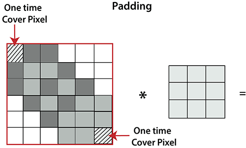
If we take a three by three filter on top of a grayscale image and do the convolving then what will happen?

It is clear from the above picture that the pixel in the corner will only get covers one time, but the middle pixel will get covered more than once. It means that we have more information on that middle pixel, so there are two downsides:

• Shrinking outputs
• Losing information on the corner of the image.

To overcome this, we have introduced padding to an image. "Padding is an additional layer which can add to the border of an image."

Pooling Layer

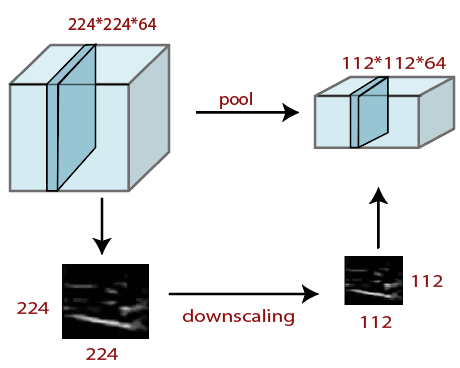
Pooling layer plays an important role in pre-processing of an image. Pooling layer reduces the number of parameters when the images are too large. Pooling is "downscaling" of the image obtained from the previous layers. It can be compared to shrinking an image to reduce its pixel density. Spatial pooling is also called downsampling or subsampling, which reduces the dimensionality of each map but retains the important information. There are the following types of spatial pooling:

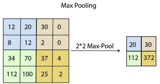
Max Pooling

Max pooling is a sample-based discretization process. Its main objective is to downscale an input representation, reducing its dimensionality and allowing for the assumption to be made about features contained in the sub-region binned.

Max pooling is done by applying a max filter to non-overlapping sub-regions of the initial representation.

Average Pooling

Down-scaling will perform through average pooling by dividing the input into rectangular pooling regions and computing the average values of each region.

Syntax

layer = averagePooling2dLayer(poolSize)
layer = averagePooling2dLayer(poolSize,Name,Value)

Sum Pooling

The sub-region for sum pooling or mean pooling are set exactly the same as for max-pooling but instead of using the max function we use sum or mean.

Fully Connected Layer

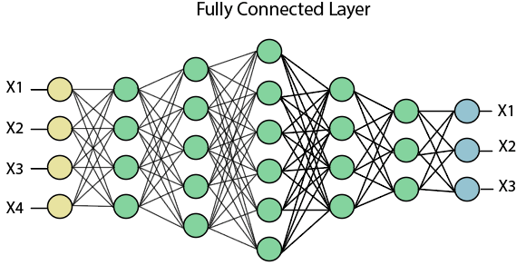
The fully connected layer is a layer in which the input from the other layers will be flattened into a vector and sent. It will transform the output into the desired number of classes by the network.

In the above diagram, the feature map matrix will be converted into the vector such as x1, x2, x3... xn with the help of fully connected layers. We will combine features to create a model and apply the activation function such as softmax or sigmoid to classify the outputs as a car, dog, truck, etc.

Ques.  Define convolutional network.

Answer

A Convolutional Neural Network (CNN) is a Deep Learning algorithm which can take in

• an input image
• assign importance (learnable weights and biases) to various aspects/objects in the image
• be able to differentiate one from the other.

Convolutional neural networks are very good at picking up on patterns in the input image, such as lines, gradients, circles, or even eyes and faces.It is a feed-forward neural network and contain many convolutional layers stacked on top of each other, each one capable of recognizing more sophisticated shapes. 

 

Ques. Write a short note on the convolutional layer.

Answer

It is a key building block which makes use of a set of learnable filters. A filter is used to detect the presence of specific features or patterns present in the original image (input). A convolution is the simple application of a filter to an input that results in an activation.

Usage:

The usage of convolutional layers in a convolutional neural network mirrors the structure of the human visual cortex, where a series of layers process an incoming image and identify progressively more complex features.

 

Ques. Describe briefly activation function, pooling and fully connected layer.

Answer

The activation function is a node that is put at the end of or in between Neural Networks. They help to decide if the neuron would fire or not.

Pooling basically reduces the number of parameters and computation in the network, controlling overfitting by progressively reducing the spatial size of the network.

There are 3 types of pooling:

• Max(take out only the maximum from a pool.)
• Min(take out only the minimum from a pool.)
• Average(take out only the average from a pool.)

In Fully Connected Layer the neurons have a complete connection to all the activations from the previous layers.

Deep Learning

What exactly is Deep Learning?

Deep Learning is a subset of Machine Learning, which on the other hand is a subset of Artificial Intelligence. Artificial Intelligence is a general term that refers to techniques that enable computers to mimic human behavior. Machine Learning represents a set of algorithms trained on data that make all of this possible.

AI. vs ML. vs DL.

Deep Learning, on the other hand, is just a type of Machine Learning, inspired by the structure of a human brain. Deep learning algorithms attempt to draw similar conclusions as humans would by continually analyzing data with a given logical structure. To achieve this, deep learning uses a multi-layered structure of algorithms called neural networks.

A typical Neural Network.

The design of the neural network is based on the structure of the human brain. Just as we use our brains to identify patterns and classify different types of information, neural networks can be taught to perform the same tasks on data.

The individual layers of neural networks can also be thought of as a sort of filter that works from gross to subtle, increasing the likelihood of detecting and outputting a correct result.

The human brain works similarly. Whenever we receive new information, the brain tries to compare it with known objects. The same concept is also used by deep neural networks.

Neural networks enable us to perform many tasks, such as clustering, classification or regression. With neural networks, we can group or sort unlabeled data according to similarities among the samples in this data. Or in the case of classification, we can train the network on a labeled dataset in order to classify the samples in this dataset into different categories.

In general, neural networks can perform the same tasks as classical algorithms of machine learning. However, it is not the other way around.

Artificial neural networks have unique capabilities that enable deep learning models to solve tasks that machine learning models can never solve.

All recent advances in artificial intelligence in recent years are due to deep learning. Without deep learning, we would not have self-driving cars, chatbots or personal assistants like Alexa and Siri. The Google Translate app would continue to be as primitive as 10 years ago (before Google switched to neural networks for this App), and Netflix or Youtube would have no idea which movies or TV series we like or dislike. Behind all these technologies are neural networks.

We can even go so far as to say that today a new industrial revolution is taking place, driven by artificial neural networks and deep learning.

At the end of the day, deep learning is the best and most obvious approach to real machine intelligence we’ve had so far.

Comparing deep learning with machine learning

SOM Algorithm and its variant

Self-Organizing Maps (SOMs) are a type of unsupervised learning algorithm used for dimensionality reduction and data visualization. SOMs transform complex, high-dimensional data into a simpler, often two-dimensional grid while preserving the relationships between data points. SOMs are a part of artificial neural networks developed by Teuvo Kohonen in the 1980s, and hence, they are sometimes referred to as Kohonen maps.

---

How SOM Works

1. Input Layer and Weight Initialization:

   • Each neuron in the SOM is associated with a weight vector of the same dimension as the input data.
   • These weights are initialized randomly or using heuristics.

2. Finding the Best Matching Unit (BMU):

   • For each input vector, the SOM calculates the similarity (e.g., Euclidean distance) between the input vector and each neuron's weight vector.
   • The neuron with the closest weight vector is called the Best Matching Unit (BMU).

3. Updating Weights:

   • The weights of the BMU and its neighboring neurons are updated to make them closer to the input vector.
   • This is done using the formula:
     W(t+1)=W(t)+α(t)⋅(X−W(t))W(t+1)
     Where:
   • W(t): Weight vector at time 𝑡
   • α(t): Learning rate 
   • X: Input vector 
   • t: Iteration count

4. Neighborhood Function:

   • Neurons closer to the BMU in the grid receive a greater update, while those farther away receive a smaller update.
   • The influence of the neighborhood decreases over time.

5. Iterative Process:

   • The algorithm iteratively updates weights for all input vectors, leading to the organization of the map.

---

Example: Clustering of Colors

Imagine we want to group a set of RGB colors using a 2D SOM.

1. Input Data: RGB color vectors (e.g., [255, 0, 0] for red, [0, 255, 0] for green, [0, 0, 255] for blue).

2. SOM Grid: A 10x10 grid of neurons is initialized. Each neuron has a weight vector corresponding to RGB values.

3. Training:

   • For each color in the dataset, the SOM finds the BMU based on the closest RGB match.
   • The BMU and its neighbors in the grid are updated to resemble the input color.

4. Result:

   • After several iterations, neurons in one part of the grid represent red shades, another part represents green shades, and yet another represents blue shades. Intermediate shades (like yellow or purple) form regions between these.

---

Applications of SOMs

1. Data Visualization: Reduce high-dimensional data to a 2D or 3D representation.
2. Clustering: Group similar data points without prior labeling.
3. Anomaly Detection: Identify unusual data patterns in network security or fraud detection.
4. Feature Extraction: Find patterns or structures in image and audio data.

---

Key Advantages

• Intuitive representation of data relationships.
• Useful for non-linear dimensionality reduction.
• Helps in exploratory data analysis.

---

Visual Representation

For the above color clustering example, the final grid would look like a smooth gradient of colors, with similar colors grouped closer together. This visually demonstrates the SOM's ability to organize and map input data onto a lower-dimensional space.

Example: A Kohonen self-organizing map is used to cluster four vectors. Let the vectors to be clustered be (1,1,0,0); (0,0,0,1); (1,0,0,0);(0,0,1,1) The maximum number of clusters to be formed is m = 2. Suppose the learning rate is n = 0.5, The neighborhood of node J is set so that only one cluster updates its weights at each step (R = 0). Initial weight matrix is [0.2 0.4 0.6 0.8] [0.9 0.7 0.5 0.3]. 

Solving the Problem Using Kohonen Self-Organizing Map (SOM)

Given:

• Input vectors: (1, 1, 0, 0), (0, 0, 0, 1), (1, 0, 0, 0), (0, 0, 1, 1)
• Clusters (m): 2
• Learning rate (n): 0.5
• Neighborhood radius (R): 0 (Only the Best Matching Unit (BMU) updates).
• Initial weight matrix:
  • Cluster 1: [0.2, 0.4, 0.6, 0.8]
  • Cluster 2: [0.9, 0.7, 0.5, 0.3]

---

Steps for Each Iteration:

1. Compute the Euclidean distance between each input vector and the weight vectors of the clusters to find the Best Matching Unit (BMU).

2. Update the BMU's weights using the formula:
   New weight = Old weight + Learning rate × (Input vector − Old weight)

3. Repeat for all input vectors, updating weights at each step.

---

Iteration-by-Iteration Solution

Initial Weights:

Cluster 1: [0.2, 0.4, 0.6, 0.8]

Cluster 2: [0.9, 0.7, 0.5, 0.3]

---

Step 1: Input Vector (1, 1, 0, 0)

1. Compute Euclidean distances:
   For Cluster 1:
   Distance = √((1 − 0.2)² + (1 − 0.4)² + (0 − 0.6)² + (0 − 0.8)²) = √(0.64 + 0.36 + 0.36 + 0.64) = √2.0
   For Cluster 2:
   Distance = √((1 − 0.9)² + (1 − 0.7)² + (0 − 0.5)² + (0 − 0.3)²) = √(0.01 + 0.09 + 0.25 + 0.09) = √0.44

   BMU: Cluster 2 (as its distance is smaller).

2. Update weights for Cluster 2:
   New weight = Old weight + 0.5 × (Input vector − Old weight)
   For Cluster 2: [0.9, 0.7, 0.5, 0.3] + 0.5 × ([1, 1, 0, 0] − [0.9, 0.7, 0.5, 0.3])
   = [0.9, 0.7, 0.5, 0.3] + [0.05, 0.15, −0.25, −0.15]
   = [0.95, 0.85, 0.25, 0.15]
   Updated weights:
   Cluster 1: [0.2, 0.4, 0.6, 0.8]
   Cluster 2: [0.95, 0.85, 0.25, 0.15]

---

Step 2: Input Vector (0, 0, 0, 1)

1. Compute Euclidean distances:
   For Cluster 1:
   Distance = √((0 − 0.2)² + (0 − 0.4)² + (0 − 0.6)² + (1 − 0.8)²) = √(0.04 + 0.16 + 0.36 + 0.04) = √0.6
   For Cluster 2:
   Distance = √((0 − 0.95)² + (0 − 0.85)² + (0 − 0.25)² + (1 − 0.15)²) = √(0.9025 + 0.7225 + 0.0625 + 0.7225) = √2.41

   BMU: Cluster 1 (as its distance is smaller).

2. Update weights for Cluster 1:
   New weight = Old weight + 0.5 × (Input vector − Old weight)
   For Cluster 1: [0.2, 0.4, 0.6, 0.8] + 0.5 × ([0, 0, 0, 1] − [0.2, 0.4, 0.6, 0.8])
   = [0.2, 0.4, 0.6, 0.8] + [−0.1, −0.2, −0.3, 0.1]
   = [0.1, 0.2, 0.3, 0.9]
   Updated weights:
   Cluster 1: [0.1, 0.2, 0.3, 0.9]
   Cluster 2: [0.95, 0.85, 0.25, 0.15]

---

Step 3: Input Vector (1, 0, 0, 0)

1. Compute Euclidean distances:
   For Cluster 1:
   Distance = √((1 − 0.1)² + (0 − 0.2)² + (0 − 0.3)² + (0 − 0.9)²) = √(0.81 + 0.04 + 0.09 + 0.81) = √1.75
   For Cluster 2:
   Distance = √((1 − 0.95)² + (0 − 0.85)² + (0 − 0.25)² + (0 − 0.15)²) = √(0.0025 + 0.7225 + 0.0625 + 0.0225) = √0.81

   BMU: Cluster 2 (as its distance is smaller).

2. Update weights for Cluster 2:
   New weight = Old weight + 0.5 × (Input vector − Old weight)
   For Cluster 2: [0.95, 0.85, 0.25, 0.15] + 0.5 × ([1, 0, 0, 0] − [0.95, 0.85, 0.25, 0.15])
   = [0.95, 0.85, 0.25, 0.15] + [0.025, −0.425, −0.125, −0.075]
   = [0.975, 0.425, 0.125, 0.075]
   Updated weights:
   Cluster 1: [0.1, 0.2, 0.3, 0.9]
   Cluster 2: [0.975, 0.425, 0.125, 0.075]

---

Step 4: Input Vector (0, 0, 1, 1)

1. Compute Euclidean distances:
   For Cluster 1:
   Distance = √((0 − 0.1)² + (0 − 0.2)² + (1 − 0.3)² + (1 − 0.9)²) = √(0.01 + 0.04 + 0.49 + 0.01) = √0.55
   For Cluster 2:
   Distance = √((0 − 0.975)² + (0 − 0.425)² + (1 − 0.125)² + (1 − 0.075)²) = √(0.950625 + 0.180625 + 0.765625 + 0.855625) = √2.75

   BMU: Cluster 1 (as its distance is smaller).

2. Update weights for Cluster 1:
   New weight = Old weight + 0.5 × (Input vector − Old weight)
   For Cluster 1: [0.1, 0.2, 0.3, 0.9] + 0.5 × ([0, 0, 1, 1] − [0.1, 0.2, 0.3, 0.9])
   = [0.1, 0.2, 0.3, 0.9] + [−0.05, −0.1, 0.35, 0.05]
   = [0.05, 0.1, 0.65, 0.95]
   Final weights:
   Cluster 1: [0.05, 0.1, 0.65, 0.95]
   Cluster 2: [0.975, 0.425, 0.125, 0.075]

---

Result

After training, the final cluster weights are:

• Cluster 1: [0.05, 0.1, 0.65, 0.95]
• Cluster 2: [0.975, 0.425, 0.125, 0.075]

These represent the centroids of the clusters formed by the SOM.