The BACKPROPAGATION Algorithm

• The BACKPROPAGATION Algorithm learns the weights for a multilayer network, given a network with a fixed set of units and interconnections. It employs gradient descent to attempt to minimize the squared error between the network output values and the target values for these outputs.
• In BACKPROPAGATION algorithm, we consider networks with multiple output units rather than single units as before, so we redefine E to sum the errors over all of the network output units.

 

where,

• outputs - is the set of output units in the network
• tkd and Okd - the target and output values associated with the kth output unit
• d - training example

Algorithm:

BACKPROPAGATION (training_example, ƞ, n_in, n_out, n_hidden )

 Each training example is a pair of the form (𝑥⃗  ,t⃗), where (𝑥⃗) is the vector of network

input values, (t⃗) and is the vector of target network output values.

ƞ is the learning rate (e.g., .05). n_i, is the number of network inputs, n_hidden the number of units in the hidden layer, and n_out the number of output units.

The input from unit i into unit j is denoted x_ji, and the weight from unit i to unit j is denoted w_ji

• Create a feed-forward network with n_i inputs, n_hidden hidden units, and n_out output units.
• Initialize all network weights to small random numbers
• Until the termination condition is met, Do

·        For each (𝑥⃗  ,t⃗), in training examples, Do 

Propagate the input forward through the network:

1.     Input the instance 𝑥⃗ , to the network and compute the output o_u of every unit u in the network.

Propagate the errors backward through the network:

Adding Momentum

Because BACKPROPAGATION is such a widely used algorithm, many variations have been developed. The most common is to alter the weight-update rule the equation below

by making the weight update on the nth iteration depend partially on the update that occurred during the (n - 1)^th iteration, as follows:

 Learning in arbitrary acyclic networks

• BACKPROPAGATION algorithm given there easily generalizes to feedforward networks of arbitrary depth. The weight update rule is retained, and the only change is to the procedure for computing δ values.
• In general, the δ, value for a unit r in layer m is computed from the δ values at the next deeper layer m + 1 according to

 

• The rule for calculating δ for any internal unit

 
Where, Downstream(r) is the set of units immediately downstream from unit r in the network: that is, all units whose inputs include the output of unit r

 Derivation of the BACKPROPAGATION Rule

• Deriving the stochastic gradient descent rule: Stochastic gradient descent involves iterating through the training examples one at a time, for each training example d descending the gradient of the error Ed with respect to this single example
• For each training example d every weight wji is updated by adding to it Δwji

Here outputs is the set of output units in the network, tk is the target value of unit k for training example d, and ok is the output of unit k given training example d.

The derivation of the stochastic gradient descent rule is conceptually straightforward, but requires keeping track of a number of subscripts and variables

• xji = the i^th input to unit j
• wji = the weight associated with the i^th input to unit j
• netj = Σi wjixji (the weighted sum of inputs for unit j )
• oj = the output computed by unit j
• tj = the target output for unit j
• σ = the sigmoid function
• outputs = the set of units in the final layer of the network
• Downstream(j) = the set of units whose immediate inputs include the output of unit j

Consider two cases: The case where unit j is an output unit for the network, and the case where j is an internal unit (hidden unit).

 

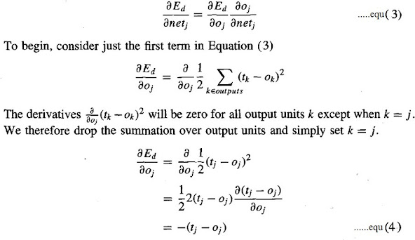
Case 1: Training Rule for Output Unit Weights.

wji can influence the rest of the network only through netj , netj can influence the network only through oj. Therefore, we can invoke the chain rule again to write

Case 2: Training Rule for Hidden Unit Weights.

• In the case where j is an internal, or hidden unit in the network, the derivation of the training rule for wji must take into account the indirect ways in which wji can influence the network outputs and hence Ed.
• For this reason, we will find it useful to refer to the set of all units immediately downstream of unit j in the network and denoted this set of units by Downstream( j).
• netj can influence the network outputs only through the units in Downstream(j). Therefore, we can write