CLR (1) Parsing

CLR refers to canonical lookahead. CLR parsing use the canonical collection of LR (1) items to build the CLR (1) parsing table. CLR (1) parsing table produces the more number of states as compare to the SLR (1) parsing.

In the CLR (1), we place the reduce node only in the lookahead symbols.

Various steps involved in the CLR (1) Parsing:

• For the given input string write a context free grammar
• Check the ambiguity of the grammar
• Add Augment production in the given grammar
• Create Canonical collection of LR (0) items
• Draw a data flow diagram (DFA)
• Construct a CLR (1) parsing table

LR (1) item

LR (1) item is a collection of LR (0) items and a look ahead symbol.

LR (1) item = LR (0) item + look ahead

The look ahead is used to determine that where we place the final item.

The look ahead always add $ symbol for the argument production.

Example

CLR ( 1 ) Grammar

1. S → AA  
2. A → aA  
3. A → b  

Add Augment Production, insert '•' symbol at the first position for every production in G and also add the lookahead.

1. S` → •S, $  
2. S  → •AA, $  
3. A  → •aA, a/b   
4. A → •b, a/b  

I0 State:

Add Augment production to the I0 State and Compute the Closure

I0 = Closure (S` → •S)

Add all productions starting with S in to I0 State because "." is followed by the non-terminal. So, the I0 State becomes

I0 = S` → •S, $
        S → •AA, $

Add all productions starting with A in modified I0 State because "." is followed by the non-terminal. So, the I0 State becomes.

I0=  S` → •S, $
        S → •AA, $
        A → •aA, a/b
        A → •b, a/b

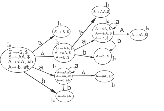
I1= Go to (I0, S) = closure (S` → S•, $) = S` → S•, $
I2= Go to (I0, A) = closure ( S → A•A, $ )

Add all productions starting with A in I2 State because "." is followed by the non-terminal. So, the I2 State becomes

I2= S → A•A, $
       A → •aA, $
       A → •b, $

I3= Go to (I0, a) = Closure ( A → a•A, a/b )

Add all productions starting with A in I3 State because "." is followed by the non-terminal. So, the I3 State becomes

I3= A → a•A, a/b
       A → •aA, a/b
       A → •b, a/b

Go to (I3, a) = Closure (A → a•A, a/b) = (same as I3)
Go to (I3, b) = Closure (A → b•, a/b) = (same as I4)

I4= Go to (I0, b) = closure ( A → b•, a/b) = A → b•, a/b
I5= Go to (I2, A) = Closure (S → AA•, $) =S → AA•, $
I6= Go to (I2, a) = Closure (A → a•A, $)

Add all productions starting with A in I6 State because "." is followed by the non-terminal. So, the I6 State becomes

I6 = A → a•A, $
       A → •aA, $
       A → •b, $

Go to (I6, a) = Closure (A → a•A, $) = (same as I6)
Go to (I6, b) = Closure (A → b•, $) = (same as I7)

I7= Go to (I2, b) = Closure (A → b•, $) = A → b•, $
I8= Go to (I3, A) = Closure (A → aA•, a/b) = A → aA•, a/b
I9= Go to (I6, A) = Closure (A → aA•, $) = A → aA•, $

Drawing DFA:

CLR (1) Parsing table:

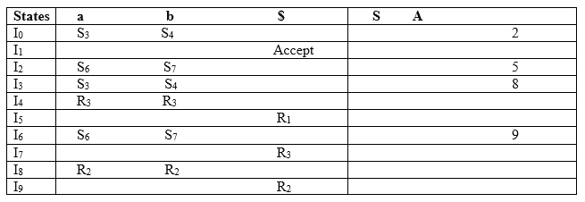
Productions are numbered as follows:

1. S  →  AA      ... (1)                                  
2.   A  → aA       ....(2)     
3.   A  →  b     ... (3)  

The placement of shift node in CLR (1) parsing table is same as the SLR (1) parsing table. Only difference in the placement of reduce node.

I4 contains the final item which drives ( A → b•, a/b), so action {I4, a} = R3, action {I4, b} = R3.
I5 contains the final item which drives ( S → AA•, $), so action {I5, $} = R1.
I7 contains the final item which drives ( A → b•,$), so action {I7, $} = R3.
I8 contains the final item which drives ( A → aA•, a/b), so action {I8, a} = R2, action {I8, b} = R2.
I9 contains the final item which drives ( A → aA•, $), so action {I9, $} = R2.