Loop Unrolling
Loop unrolling is a loop transformation technique that helps to optimize the execution time of a program. We basically remove or reduce iterations. Loop unrolling increases the program’s speed by eliminating loop control instruction and loop test instructions.
// This program does not uses loop unrolling.
#include<stdio.h>
int main(void)
{
for (int
i=0; i<5; i++)
printf("Hello\n"); //print hello 5 times
return
0;
}
// This program uses loop unrolling.
#include<stdio.h>
int main(void)
{
//
unrolled the for loop in program 1
printf("Hello\n");
printf("Hello\n");
printf("Hello\n");
printf("Hello\n");
printf("Hello\n");
return
0;
}
Illustration:
Program 2 is more efficient than program 1 because in program 1 there is a need
to check the value of i and increment the value of i every time round the loop.
So small loops like this or loops where there is fixed number of iterations are
involved can be unrolled completely to reduce the loop overhead.
Advantages:
·
Increases
program efficiency.
·
Reduces
loop overhead.
·
If
statements in loop are not dependent on each other, they can be executed in
parallel.
Disadvantages:
·
Increased
program code size, which can be undesirable.
·
Possible
increased usage of register in a single iteration to store temporary variables
which may reduce performance.
·
Apart
from very small and simple codes, unrolled loops that contain branches are even
slower than recursion.
Loop Jamming
Loop jamming or loop fusion is a technique for combining two similar loops into one, thus reducing loop overhead by a factor of 2. For example, the following C code:
for
(i=1;i<=100;i++)
x[i]=y[i]*8;
for
(i=1;i<=100;i++)
z[i]=x[i]*y[i];
for
(i=1;i<=100;i++) {
x[i]=y[i]*8;
z[i]=x[i]*y[i]; };
The loop overhead is reduced, resulting in a
speed-up in execution, as well as a reduction in code space. Once again,
instructions are exposed for parallel execution.
The conditions for performing this
optimization are that the loop indices be the same, and the computations in one
loop cannot depend on the computations in the other loop.
Sometimes loops may be fused when one loop
index is a subset of the other:
FOR I := 1 TO10000 DO
A[I] := 0
FOR J := 1 TO 5000 DO
B[J] := 0
can be replaced by
FOR I := 1 to 10000 DO
IF
I <= 5000 THEN B[I] := 0
A[I]
:= 0
Here, a test has been added
to compute the second loop within the first. The loop must execute many times
for this optimization to be worthwhile.
Cross-Jump
Elimination If the same code appears in more than
one case in a case or switch statement, then it is better to combine the
cases
into one. This eliminates an additional jump or cross jump. For example, the
following code :
switch (x)
{
case 0: x=x+1;
break;
case 1: x=x*2;
break;
case 2: x=x+1;
break;
case 3: x=2;
break;
};
can be replaced by
switch (x)
{
case 0:
case 2: x=x+1;
break;
case 1: x=x*2;
break;
case 3: x=2;
break;
};
LOOPS
IN FLOW GRAPH
A
graph representation of three-address statements, called a flow graph, is
useful for understanding code-generation algorithms, even if the graph is not
explicitly constructed by a code-generation algorithm. Nodes in the flow graph
represent computations, and the edges represent the flow of control.
Dominators: In
a flow graph, a node d dominates node n, if every path from initial node of the
flow graph to n goes through d. This will be denoted by d dom n. Every initial
node dominates all the remaining nodes in the flow graph and the entry of a
loop dominates all nodes in the loop. Similarly, every node dominates itself.
Example:
*In the flow graph below,
*Initial node,node1 dominates every node.
*node 2 dominates itself
*node 3 dominates all but 1 and 2. *node 4
dominates all but 1,2 and 3.
*node 5 and 6 dominates only themselves, since
flow of control can skip around either by goin through the other.
*node 7 dominates 7,8 ,9 and 10. *node 8
dominates 8,9 and 10.
*node 9 and 10 dominates only themselves.

Fig.
(a) Flow graph (b) Dominator tree
The way of presenting dominator information
is in a tree, called the dominator tree, in which
• The initial node is the root.
• The parent of each other node is its
immediate dominator.
• Each node d dominates only its descendants in the tree.
The existence of dominator tree follows from
a property of dominators; each node has a unique immediate dominator in that is
the last dominator of n on any path from the initial node to n. In terms of the
dom relation, the immediate dominator m has the property is d=!n and d dom n,
then d dom m.
***
D(1)={1}
D(2)={1,2}
D(3)={1,3}
D(4)={1,3,4}
D(5)={1,3,4,5}
D(6)={1,3,4,6}
D(7)={1,3,4,7}
D(8)={1,3,4,7,8}
D(9)={1,3,4,7,8,9}
D(10)={1,3,4,7,8,10}
Natural
Loops: One application of dominator information is in determining the loops
of a flow graph suitable for improvement. There are two essential properties of
loops:
·
A
loop must have a single entry-point, called the header. This entry
point-dominates all nodes in the loop, or it would not be the sole entry to the
loop.
·
There
must be at least one way to iterate the loop(i.e.)at least one path back to the
header One way to find all the loops in a flow graph is to search for edges in
the flow graph whose heads dominate their tails. If a→b is an edge, b is the
head and a is the tail. These types of edges are called as back edges.
Example:
In the above graph,
7→4 4 DOM 7
10 →7 7 DOM 10
4→3
8→3
9 →1
The
above edges will form loop in flow graph. Given a back edge n → d, we define
the natural loop of the edge to be d plus the set of nodes that can reach n
without going through d. Node d is the header of the loop.
Algorithm: Constructing the natural loop of a
back edge.
Input: A flow graph G and a back edge n→d.
Output: The set loop consisting of all nodes in the
natural loop n→d.
Method: Beginning with node n, we consider each node
m*d that we know is in loop, to make sure that m’s predecessors are also placed
in loop. Each node in loop, except for d, is placed once
on
stack, so its predecessors will be examined. Note that because d is put in the
loop initially, we never examine its predecessors, and thus find only those
nodes that reach n without going through d.
Procedure insert(m);
if m is not in loop then begin loop := loop U {m};
push m onto stack end;
stack
: = empty;
loop : = {d}; insert(n);
while stack is not empty do begin
pop m, the first element of stack, off stack;
for
each predecessor p of m do insert(p)
end
Inner loops: If we use the natural
loops as “the loops”, then we have the useful property that unless two loops
have the same header, they are either disjointed or one is entirely contained
in the other.
Thus, neglecting loops with the same header
for the moment, we have a natural notion of inner loop: one that contains no
other loop.
When two natural loops have the same header,
but neither is nested within the other, they are combined and treated as a
single loop.
Pre-Headers: Several transformations require us to move statements “before the header”. Therefore, begin treatment of a loop L by creating a new block, called the preheader. The pre-header has only the header as successor, and all edges which formerly entered the header of L from outside L instead enter the pre-header. Edges from inside loop L to the header are not changed. Initially the pre-header is empty, but transformations on L may place statements in it.
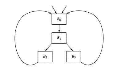
Fig. Two loops with the same header

Fig. Introduction of the preheader
Reducible
flow graphs: Reducible
flow graphs are special flow graphs, for which several code optimization
transformations are especially easy to perform, loops are unambiguously
defined, dominators can be easily calculated, data flow analysis problems can
also be solved efficiently. Exclusive use of structured flow-of-control
statements such as if-then-else, while-do, continue, and break statements
produces programs whose flow graphs are always reducible.
The most important properties of reducible
flow graphs are that
- There are no umps into the middle of loops from outside;
- The only entry to a loop is through its header
Definition: A flow graph G is reducible if and only if we can partition the edges into two disjoint groups, forward edges and back edges, with the following properties.
- The forward edges from an acyclic graph in which every node can be reached from initial node of G.
- The back edges consist only of edges where heads dominate theirs tails.
Example: The above flow graph is
reducible. If we know the relation DOM for a flow graph, we can find and remove
all the back edges. The remaining edges are forward edges. If the forward edges
form an acyclic graph, then we can say the flow graph reducible. In the above
example remove the five back edges 4→3, 7→4, 8→3, 9→1 and 10→7 whose heads
dominate their tails, the remaining graph is acyclic.
Viable Prefixes and
Handle in LR Parsing
let’s
start from the basic of Bottom up Parsing
Consider the grammar S→XXS→XX X→aX∣bX→aX∣b
Now, consider a string in L(S)L(S) say aabb. We can parse it as follows by left most derivation – replacing the left most non-terminal in each step, or right most derivation – replacing the rightmost non-terminal in each step.
S→XXS→XX
→aXX→aXX
→aaXX→aaXX
→aabX→aabX
→aabb→aabb
S→XXS→XX
→Xb→Xb
→aXb→aXb
→aaXb→aaXb
→aabb→aabb
Here, the rightmost-derivation is used in bottom-up parsing.
Any
string derivable from the start symbol is a sentential form — it becomes a
sentence if it contains only terminals
- A sentential form that occurs in the leftmost derivation of some sentence is called left-sentential form
- A sentential form that occurs in the rightmost derivation of some sentence is called right-sentential form
Consider the string aabb again. We will see a
method to parse this:
1. Scan the input from left to
right and see if any substring matches the RHS of any production. If so,
replace that substring by the LHS of the production.
So,
for “aabb” we do as follows
- ‘a’ “abb” – No RHS matches ‘a’
- ‘aa’ “bb” – No RHS matches ‘a’ or ‘aa’
- ‘aab’ “b” – RHS of X→bX→b matches ‘b’ (first b from left) and so we write as
- aaXb
- ‘aaX’ “b” – RHS of X→aXX→aX matches “aX” and so we write as
- aXb – Again RHS of X→aXX→aX matches “aX” and we get
- Xb – RHS of X→bX→b matches “b” and we get
- XX – RHS of S→XXS→XX matches XX and we get
- S – the start symbol.
Now
what we did here is nothing but a bottom-up parsing. Bottom-up because we
started from the string and not from the grammar. Here, we applied a sequence
of reductions, which are as follows:
1. aabb→aaXb→aXb→Xb→XX→Saabb→aaXb→aXb→Xb→XX→S
If we go up and see the Rightmost derivation
of the string “aabb”, what we got is the same but in REVERSE order. i.e., our
bottom up parsing is doing reverse of the RIGHTMOST derivation. So, we can call
it an LRLR parser – LL for scanning the
input from Left side and RR for doing a
Rightmost derivation.
In
our parsing we substituted the RHS of a production at each step. This
substituted “substring” is called a HANDLE and are shown in BOLD below.
1. aabb →→ aaXb →→ aXb →→ Xb →→ XX →→ S
Formally
a handle is defined as (Greek letters used to denote a string of terminals and
non-terminals)
A
handle of a right sentential form ‘γγ’ (γ=αδβ(γ=αδβ) is a production E→δE→δ and a position
in γγ where δδ can be found and
substituted by EE to get the previous
step in the right most derivation of γγ — previous and not
“next” because we are doing rightmost derivation in REVERSE. Handle can be
given as a production or just the RHS of a production.
The
handle is not necessarily starting from the left most position as clear from
the above example. There is importance to the input string which occurs to the
left of the handle. For example, for the handles of “aabb”, we can have the
following set of prefixes
aabb {a,aa,aab}{a,aa,aab}
aaXb {a,aa,aaX}{a,aa,aaX}
aXb {a,aX}{a,aX}
Xb {X,Xb}{X,Xb}
XX {X,XX}{X,XX}
These
set of prefixes are called Viable Prefixes. Formally
Viable
prefixes are the prefixes of right sentential forms that do not extend beyond
the end of its handle. i.e., a viable prefix either has no handle or just one
possible handle on the extreme RIGHT which can be reduced.
We
will see later that viable prefixes can also be defined as the set of prefixes
of the right-sentential form that can appear on the stack of a shift-reduce
parser. Also, the set of all viable prefixes of a context-free language is a
REGULAR LANGUAGE. i.e., viable prefixes can be recognized by using a FINITE
AUTOMATA. Using this FINITE AUTOMATA and a stack we get the power of a Push
Down Automata and that is how we can parse context-free languages.
PEEPHOLE OPTIMIZATION
A statement-by-statement code-generations strategy often produces target code that contains redundant instructions and suboptimal constructs. The quality of such target code can be improved by applying “optimizing” transformations to the target program.
A simple but effective technique for improving the target code is peephole optimization, a method for trying to improving the performance of the target program by examining a short sequence of target instructions (called the peephole) and replacing these instructions by a shorter or faster sequence, whenever possible.
The peephole is a small, moving window on the target program. The code in the peephole need not be contiguous, although some implementations do require this. It is characteristic of peephole optimization that each improvement may spawn opportunities for additional improvements.
Characteristics of peephole optimizations:
- Redundant-instructions elimination
- Unreachable
- Flow-of-control optimizations
- Algebraic simplifications
- Use of machine idioms
1. Redundant Loads And Stores: If we see the instructions
sequence
(1) MOV R0,a
(2) MOV a,R0
we
can delete instructions (2) because whenever (2) is executed. (1) will ensure
that the value of a is already in register R0.If (2) had a label we could not
be sure that (1) was always executed immediately before (2) and so we could not
remove (2).
2.
Unreachable Code: Another opportunity for peephole
optimizations is the removal of unreachable instructions. An unlabeled
instruction immediately following an unconditional jump may be removed. This
operation can be repeated to eliminate a sequence of instructions. For example,
for debugging purposes, a large program may have within it certain segments
that are executed only if a variable debug is 1. In C, the source code might
look like:
#define
debug 0
….
If
(debug) {
Print
debugging information
}
In the intermediate representations the
if-statement may be translated as:
If
debug =1 goto L1 goto L2
L1:
print debugging information L2: ………………………… (a)
One
obvious peephole optimization is to eliminate jumps over jumps. Thus, no matter
what the value of debug; (a) can be replaced by:
If
debug ≠1 goto L2
Print
debugging information
L2: …………………………… (b)
If
debug ≠0 goto L2
Print
debugging information
L2: …………………………… (c)
As
the argument of the statement of (c) evaluates to a constant true it can be
replaced
By
goto L2. Then all the statement that print debugging aids are manifestly
unreachable and can be eliminated one at a time.
3.
Flows-Of-Control Optimizations: The unnecessary jumps can
be eliminated in either the intermediate code or the target code by the
following types of peephole optimizations. We can replace the jump
sequence
goto
L1
….
L1: gotoL2 (d)
by the sequence
goto
L2
….
L1: goto L2
If
there are now no jumps to L1, then it may be possible to eliminate the
statement L1:goto L2 provided it is preceded by an unconditional jump
.Similarly, the sequence
if
a < b goto L1
….
L1:
goto L2 (e)
can be replaced by
If
a < b goto L2
….
L1:
goto L2
Ø Finally, suppose there is
only one jump to L1 and L1 is preceded by an unconditional goto. Then the
sequence
goto
L1
L1:
if a < b goto L2 (f) L3:
may be replaced by
If
a < b goto L2
goto
L3
…….
L3:
While
the number of instructions in(e) and (f) is the same, we sometimes skip the
unconditional jump in (f), but never in (e). Thus (f) is superior to (e) in
execution time
4.
Algebraic Simplification: There is no end to
the amount of algebraic simplification that can be attempted through peephole
optimization. Only a few algebraic identities occur frequently enough that it
is worth considering implementing them. For example, statements such as
x := x+0 or
x
:= x * 1
are
often produced by straightforward intermediate code-generation algorithms, and
they can be eliminated easily through peephole optimization.
5.
Reduction in Strength: Reduction in strength replaces
expensive operations by equivalent cheaper ones on the target machine. Certain
machine instructions are considerably cheaper than others and can often be used
as special cases of more expensive operators.
For example, x² is invariably cheaper to implement as
x*x than as a call to an exponentiation routine. Fixed-point multiplication or
division by a power of two is cheaper to implement as a shift. Floating-point
division by a constant can be implemented as multiplication by a constant,
which may be cheaper.
X2 → X*X
6.
Use of Machine Idioms: The target machine may have hardware
instructions to implement certain specific operations efficiently. For example,
some machines have auto-increment and auto-decrement addressing modes. These
add or subtract one from an operand before or after using its value. The use of
these modes greatly improves the quality of code when pushing or popping a
stack, as in parameter passing. These modes can also be used in code for
statements like i : =i+1.
i:=i+1
→ i++
i:=i-1
→ i- -


No comments:
Post a Comment