IP6

IP v6 was developed by Internet Engineering Task Force (IETF) to deal with the problem of IP v4 exhaustion. IP v6 is 128-bits address having an address space of 2^128, which is way bigger than IPv4. In IPv6 we use Colon-Hexa representation. There are 8 groups and each group represents 2 Bytes.

In IPv6 representation, we have three addressing methods :

Unicast

Multicast

Anycast

Unicast Address: Unicast Address identifies a single network interface. A packet sent to unicast address is delivered to the interface identified by that address.

Multicast Address: Multicast Address is used by multiple hosts, called as Group, acquires a multicast destination address. These hosts need not be geographically together. If any packet is sent to this multicast address, it will be distributed to all interfaces corresponding to that multicast address.

Anycast Address: Anycast Address is assigned to a group of interfaces. Any packet sent to anycast address will be delivered to only one member interface (mostly nearest host possible).

Note : Broadcast is not defined in IPv6.

Types of IPv6 address:

We have 128 bits in IPv6 address but by looking at first few bits we can identify what type of address it is.

Note : In IPv6, all 0’s and all 1’s can be assigned to any host, there is not any restriction like IPv4.

Provider based Unicast address :

These are used for global communication.

First 3 bits identifies it as of this type.

Registry Id (5-bits) : Registry Id identifies the region to which it belongs. Out of 32 (i.e. 2^5), only 4 registry id’s are being used.

Provider Id : Depending on the number of service providers that operates under a region, certain bits will be allocated to Provider Id field. This field need not be fixed. Let’s say if Provider Id = 10 bits then Subscriber Id will be 56 – 10 = 46 bits.

Subscriber Id : After Provider Id is fixed, remaining part can be used by ISP as normal IP address.

Intra Subscriber : This part can be modified as per need of organization that is using the service.

Geography based Unicast address :

Global routing prefix : Global routing prefix contains all the details of Latitude and Longitude. As of now, it is not being used. In Geography based Unicast address routing will be based on location.

Interface Id : In IPv6, instead of using Host Id, we use the term Interface Id.

Some special addresses:

Unspecified –

Loopback –

IPv4 Compatible –

IPv4 mapped –

Local Unicast Addresses :

There are two types of Local Unicast addresses defined- Link local and Site Local.

Link local address:

Link local address is used for addressing on a single link. It can also be used to communicate with nodes on the same link. Link local address always begins with 1111111010 (i.e. FE80). Router will not forward any packet with Link local address.

Site local address:

Site local addresses are equivalent to private IP address in IPv4. Likely, some address space is reserved, which can only be routed within an organization. First 10-bits are set to 1111111011, which is why Site local addresses always begin with FEC0. Following 32 bits are Subnet ID, which can be used to create subnet within organization. Node address is used to uniquely identify the link; therefore, we use 48-bits MAC address here.

Congestion control algorithms

Congestion control refers to the techniques used to control or prevent congestion. Congestion control techniques can be broadly classified into two categories:  

 

Open Loop Congestion Control

Open loop congestion control policies are applied to prevent congestion before it happens. The congestion control is handled either by the source or the destination. 

Policies adopted by open loop congestion control – 

1. Retransmission Policy : 
   It is the policy in which the retransmission of the packets are taken care. If the sender feels that a sent packet is lost or corrupted, the packet needs to be retransmitted. This transmission may increase the congestion in the network. 
   To prevent congestion, retransmission timers must be designed to prevent congestion and also able to optimize efficiency. 
    
2. Window Policy : 
   The type of window at the sender side may also affect the congestion. Several packets in the Go-back-n window are resent, although some packets may be received successfully at the receiver side. This duplication may increase the congestion in the network and make it worse. 
   Therefore, a Selective repeat window should be adopted as it sends the specific packet that may have been lost. 
    
3. Discarding Policy : 
   A good discarding policy adopted by the routers is that the routers may prevent congestion and at the same time partially discards the corrupted or less sensitive package and also able to maintain the quality of a message. 
   In case of audio file transmission, routers can discard less sensitive packets to prevent congestion and also maintain the quality of the audio file. 
    
4. Acknowledgment Policy : 
   Since acknowledgments are also part of the load in the network, the acknowledgment policy imposed by the receiver may also affect congestion. Several approaches can be used to prevent congestion related to acknowledgment. 
   The receiver should send an acknowledgment for N packets rather than sending an acknowledgment for a single packet. The receiver should send an acknowledgment only if it has to send a packet or a timer expires. 
    
5. Admission Policy : 
   In admission policy a mechanism should be used to prevent congestion. Switches in a flow should first check the resource requirement of a network flow before transmitting it further. If there is a chance of a congestion or there is a congestion in the network, router should deny establishing a virtual network connection to prevent further congestion.

All the above policies are adopted to prevent congestion before it happens in the network. 

 

Closed Loop Congestion Control

Closed loop congestion control technique is used to treat or alleviate congestion after it happens. Several techniques are used by different protocols; some of them are: 

 

1. Backpressure : 
   Backpressure is a technique in which a congested node stop receiving packet from upstream node. This may cause the upstream node or nodes to become congested and rejects receiving data from above nodes. Backpressure is a node-to-node congestion control technique that propagate in the opposite direction of data flow. The backpressure technique can be applied only to virtual circuit where each node has information of its above upstream node. 

1. In above diagram the 3rd node is congested and stops receiving packets as a result 2nd node may be get congested due to slowing down of the output data flow. Similarly 1st node may get congested and informs the source to slow down. 
    

2. Choke Packet Technique : 
   Choke packet technique is applicable to both virtual networks as well as datagram subnets. A choke packet is a packet sent by a node to the source to inform it of congestion. Each router monitor its resources and the utilization at each of its output lines. whenever the resource utilization exceeds the threshold value which is set by the administrator, the router directly sends a choke packet to the source giving it a feedback to reduce the traffic. The intermediate nodes through which the packets has traveled are not warned about congestion.  

1. Implicit Signaling : 
   In implicit signaling, there is no communication between the congested nodes and the source. The source guesses that there is congestion in a network. For example when sender sends several packets and there is no acknowledgment for a while, one assumption is that there is a congestion. 
    
2. Explicit Signaling : 
   In explicit signaling, if a node experiences congestion it can explicitly sends a packet to the source or destination to inform about congestion. The difference between choke packet and explicit signaling is that the signal is included in the packets that carry data rather than creating different packet as in case of choke packet technique. 
   Explicit signaling can occur in either forward or backward direction. 
• Forward Signaling : In forward signaling signal is sent in the direction of the congestion. The destination is warned about congestion. The receiver in this case adopt policies to prevent further congestion.
• Backward Signaling : In backward signaling signal is sent in the opposite direction of the congestion. The source is warned about congestion and it needs to slow down.

3. When too many packets are present in the network it causes packet delay and loss of packet which degrades the performance of the system. This situation is called congestion.

   The network layer and transport layer share the responsibility for handling congestions. One of the most effective ways to control congestion is trying to reduce the load that transport layer is placing on the network. To maintain this, the network and transport layers have to work together.

   

   With too much traffic, performance drops sharply.

   There are two types of Congestion control algorithms, which are as follows −

   • Leaky Bucket Algorithm
   • Token Bucket Algorithm

Leaky Bucket Algorithm

Let see the working condition of Leaky Bucket Algorithm −

Leaky Bucket Algorithm mainly controls the total amount and the rate of the traffic sent to the network.

Step 1 − Let us imagine a bucket with a small hole at the bottom where the rate at which water is poured into the bucket is not constant and can vary but it leaks from the bucket at a constant rate.

Step 2 − So (up to water is present in the bucket), the rate at which the water leaks does not depend on the rate at which the water is input to the bucket.

Step 3 − If the bucket is full, additional water that enters into the bucket that spills over the sides and is lost.

Step 4 − Thus the same concept applied to packets in the network. Consider that data is coming from the source at variable speeds. Suppose that a source sends data at 10 Mbps for 4 seconds. Then there is no data for 3 seconds. The source again transmits data at a rate of 8 Mbps for 2 seconds. Thus, in a time span of 8 seconds, 68 Mb data has been transmitted.

That’s why if a leaky bucket algorithm is used, the data flow would be 8 Mbps for 9 seconds. Thus, the constant flow is maintained.

Token Bucket Algorithm

The leaky bucket algorithm enforces output patterns at the average rate, no matter how busy the traffic is. So, to deal with the more traffic, we need a flexible algorithm so that the data is not lost. One such approach is the token bucket algorithm.

Let us understand this algorithm step wise as given below −

• Step 1 − In regular intervals tokens are thrown into the bucket f.

• Step 2 − The bucket has a maximum capacity f.

• Step 3 − If the packet is ready, then a token is removed from the bucket, and the packet is sent.

• Step 4 − Suppose, if there is no token in the bucket, the packet cannot be sent.

Example

Let us understand the Token Bucket Algorithm with an example −

In figure (a) the bucket holds two tokens, and three packets are waiting to be sent out of the interface.

In Figure (b) two packets have been sent out by consuming two tokens, and 1 packet is still left.

When compared to Leaky bucket the token bucket algorithm is less restrictive that means it allows more traffic. The limit of busyness is restricted by the number of tokens available in the bucket at a particular instant of time.

The implementation of the token bucket algorithm is easy − a variable is used to count the tokens. For every t seconds the counter is incremented and then it is decremented whenever a packet is sent. When the counter reaches zero, no further packet is sent out.

This is shown in below given diagram −

Routing

Routing algorithm

• In order to transfer the packets from source to the destination, the network layer must determine the best route through which packets can be transmitted.
• Whether the network layer provides datagram service or virtual circuit service, the main job of the network layer is to provide the best route. The routing protocol provides this job.
• The routing protocol is a routing algorithm that provides the best path from the source to the destination. The best path is the path that has the "least-cost path" from source to the destination.
• Routing is the process of forwarding the packets from source to the destination but the best route to send the packets is determined by the routing algorithm.

Classification of a Routing algorithm

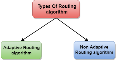
The Routing algorithm is divided into two categories:

• Adaptive Routing algorithm
• Non-adaptive Routing algorithm

---

Adaptive Routing algorithm

• An adaptive routing algorithm is also known as dynamic routing algorithm.
• This algorithm makes the routing decisions based on the topology and network traffic.
• The main parameters related to this algorithm are hop count, distance and estimated transit time.

An adaptive routing algorithm can be classified into three parts:

• Centralized algorithm: It is also known as global routing algorithm as it computes the least-cost path between source and destination by using complete and global knowledge about the network. This algorithm takes the connectivity between the nodes and link cost as input, and this information is obtained before actually performing any calculation. Link state algorithm is referred to as a centralized algorithm since it is aware of the cost of each link in the network.
• Isolation algorithm: It is an algorithm that obtains the routing information by using local information rather than gathering information from other nodes.
• Distributed algorithm: It is also known as decentralized algorithm as it computes the least-cost path between source and destination in an iterative and distributed manner. In the decentralized algorithm, no node has the knowledge about the cost of all the network links. In the beginning, a node contains the information only about its own directly attached links and through an iterative process of calculation computes the least-cost path to the destination. A Distance vector algorithm is a decentralized algorithm as it never knows the complete path from source to the destination, instead it knows the direction through which the packet is to be forwarded along with the least cost path.

---

Non-Adaptive Routing algorithm

• Non Adaptive routing algorithm is also known as a static routing algorithm.
• When booting up the network, the routing information stores to the routers.
• Non Adaptive routing algorithms do not take the routing decision based on the network topology or network traffic.

The Non-Adaptive Routing algorithm is of two types:

Flooding: In case of flooding, every incoming packet is sent to all the outgoing links except the one from it has been reached. The disadvantage of flooding is that node may contain several copies of a particular packet.

Random walks: In case of random walks, a packet sent by the node to one of its neighbors randomly. An advantage of using random walks is that it uses the alternative routes very efficiently.

Differences b/w Adaptive and Non-Adaptive Routing Algorithm

Basis Of Comparison	Adaptive Routing algorithm	Non-Adaptive Routing algorithm
Define	Adaptive Routing algorithm is an algorithm that constructs the routing table based on the network conditions.	The Non-Adaptive Routing algorithm is an algorithm that constructs the static table to determine which node to send the packet.
Usage	Adaptive routing algorithm is used by dynamic routing.	The Non-Adaptive Routing algorithm is used by static routing.
Routing decision	Routing decisions are made based on topology and network traffic.	Routing decisions are the static tables.
Categorization	The types of adaptive routing algorithm, are Centralized, isolation and distributed algorithm.	The types of Non Adaptive routing algorithm are flooding and random walks.
Complexity	Adaptive Routing algorithms are more complex.	Non-Adaptive Routing algorithms are simple.

Distance Vector Routing Algorithm

• The Distance vector algorithm is iterative, asynchronous and distributed.
  • Distributed: It is distributed in that each node receives information from one or more of its directly attached neighbors, performs calculation and then distributes the result back to its neighbors.
  • Iterative: It is iterative in that its process continues until no more information is available to be exchanged between neighbors.
  • Asynchronous: It does not require that all of its nodes operate in the lock step with each other.
• The Distance vector algorithm is a dynamic algorithm.
• It is mainly used in ARPANET, and RIP.
• Each router maintains a distance table known as Vector.

Three Keys to understand the working of Distance Vector Routing Algorithm:

• Knowledge about the whole network: Each router shares its knowledge through the entire network. The Router sends its collected knowledge about the network to its neighbors.
• Routing only to neighbors: The router sends its knowledge about the network to only those routers which have direct links. The router sends whatever it has about the network through the ports. The information is received by the router and uses the information to update its own routing table.
• Information sharing at regular intervals: Within 30 seconds, the router sends the information to the neighboring routers.

Distance Vector Routing Algorithm

Let d_x(y) be the cost of the least-cost path from node x to node y. The least costs are related by Bellman-Ford equation,

dx(y) = minv{c(x,v) + dv(y)}

Where the minv is the equation taken for all x neighbors. After traveling from x to v, if we consider the least-cost path from v to y, the path cost will be c(x,v)+d_v(y). The least cost from x to y is the minimum of c(x,v)+d_v(y) taken over all neighbors.

With the Distance Vector Routing algorithm, the node x contains the following routing information:

• For each neighbor v, the cost c(x,v) is the path cost from x to directly attached neighbor, v.
• The distance vector x, i.e., D_x = [ D_x(y) : y in N ], containing its cost to all destinations, y, in N.
• The distance vector of each of its neighbors, i.e., D_v = [ D_v(y) : y in N ] for each neighbor v of x.

Distance vector routing is an asynchronous algorithm in which node x sends the copy of its distance vector to all its neighbors. When node x receives the new distance vector from one of its neighboring vector, v, it saves the distance vector of v and uses the Bellman-Ford equation to update its own distance vector. The equation is given below:

dx(y) = minv{ c(x,v) + dv(y)}     for each node y in N

The node x has updated its own distance vector table by using the above equation and sends its updated table to all its neighbors so that they can update their own distance vectors.

Algorithm

At each node x,
Initialization

for all destinations y in N:
Dx(y) = c(x,y)     // If y is not a neighbor then c(x,y) = ∞
for each neighbor w
Dw(y) = ?     for all destination y in N.
for each neighbor w
send distance vector Dx = [ Dx(y)  : y in N ] to w
loop
  wait(until I receive any distance vector from some neighbor w)
  for each y in N:
  Dx(y) = minv{c(x,v)+Dv(y)}
If Dx(y) is changed for any destination y
Send distance vector Dx = [ Dx(y) : y in N ] to all neighbors
forever

Note: In Distance vector algorithm, node x update its table when it either see any cost change in one directly linked nodes or receives any vector update from some neighbor.

Let's understand through an example:

Sharing Information

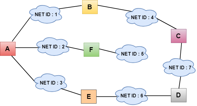
• In the above figure, each cloud represents the network, and the number inside the cloud represents the network ID.
• All the LANs are connected by routers, and they are represented in boxes labeled as A, B, C, D, E, F.
• Distance vector routing algorithm simplifies the routing process by assuming the cost of every link is one unit. Therefore, the efficiency of transmission can be measured by the number of links to reach the destination.
• In Distance vector routing, the cost is based on hop count.

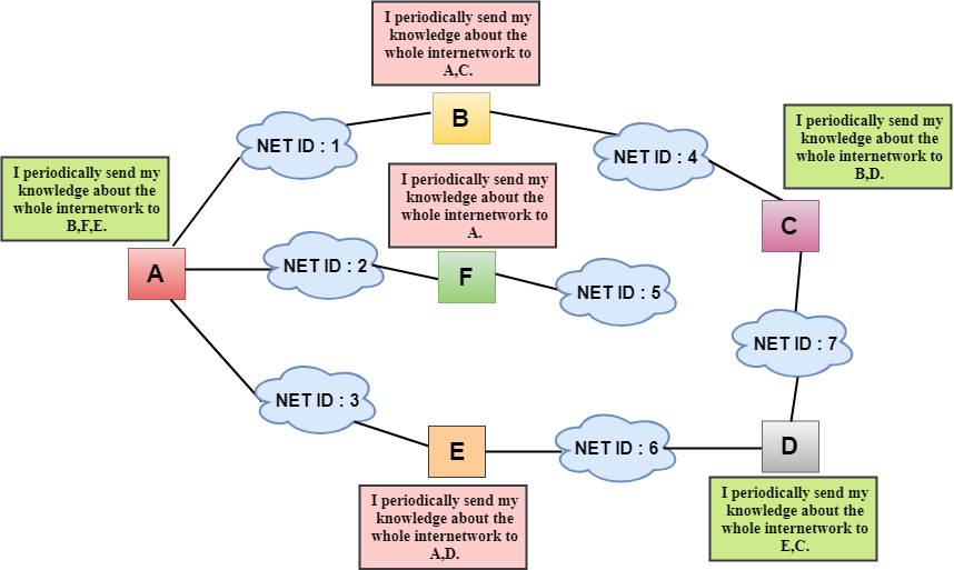
In the above figure, we observe that the router sends the knowledge to the immediate neighbors. The neighbors add this knowledge to their own knowledge and sends the updated table to their own neighbors. In this way, routers get its own information plus the new information about the neighbors.

Routing Table

Two process occurs:

• Creating the Table
• Updating the Table

Creating the Table

Initially, the routing table is created for each router that contains atleast three types of information such as Network ID, the cost and the next hop.

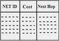
• NET ID: The Network ID defines the final destination of the packet.
• Cost: The cost is the number of hops that packet must take to get there.
• Next hop: It is the router to which the packet must be delivered.

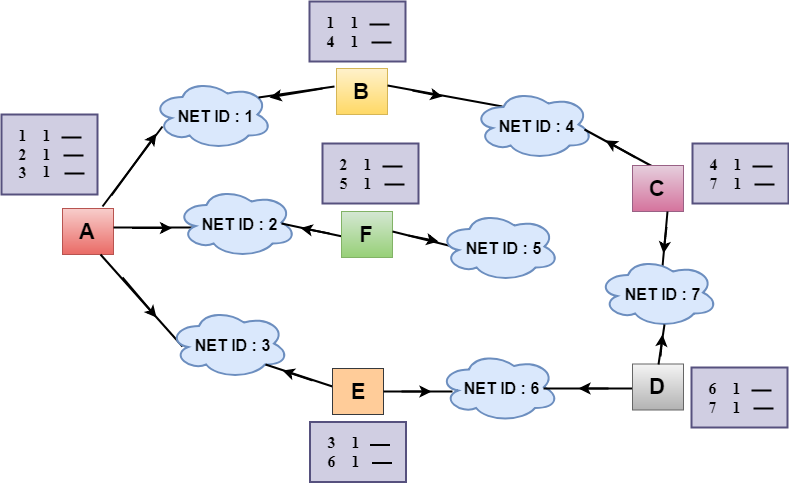
• In the above figure, the original routing tables are shown of all the routers. In a routing table, the first column represents the network ID, the second column represents the cost of the link, and the third column is empty.
• These routing tables are sent to all the neighbors.

For Example:

A sends its routing table to B, F & E.  

B sends its routing table to A & C.  

C sends its routing table to B & D.  

D sends its routing table to E & C.  

E sends its routing table to A & D.  

F sends its routing table to A. 

Updating the Table

• When A receives a routing table from B, then it uses its information to update the table.
• The routing table of B shows how the packets can move to the networks 1 and 4.
• The B is a neighbor to the A router, the packets from A to B can reach in one hop. So, 1 is added to all the costs given in the B's table and the sum will be the cost to reach a particular network.

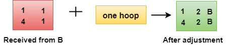
• After adjustment, A then combines this table with its own table to create a combined table.

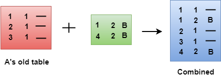
• The combined table may contain some duplicate data. In the above figure, the combined table of router A contains the duplicate data, so it keeps only those data which has the lowest cost. For example, A can send the data to network 1 in two ways. The first, which uses no next router, so it costs one hop. The second requires two hops (A to B, then B to Network 1). The first option has the lowest cost, therefore it is kept and the second one is dropped.

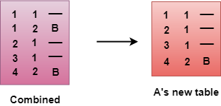
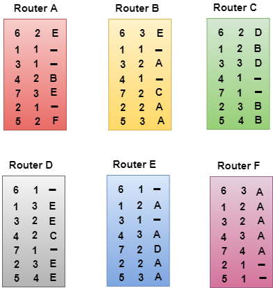
• The process of creating the routing table continues for all routers. Every router receives the information from the neighbors, and update the routing table.

Final routing tables of all the routers are given below:

Link State Routing

Link state routing is a technique in which each router shares the knowledge of its neighborhood with every other router in the internetwork.

The three keys to understand the Link State Routing algorithm:

• Knowledge about the neighborhood: Instead of sending its routing table, a router sends the information about its neighborhood only. A router broadcast its identities and cost of the directly attached links to other routers.
• Flooding: Each router sends the information to every other router on the internetwork except its neighbors. This process is known as Flooding. Every router that receives the packet sends the copies to all its neighbors. Finally, each and every router receives a copy of the same information.
• Information sharing: A router sends the information to every other router only when the change occurs in the information.

Link State Routing has two phases:

Reliable Flooding

• Initial state: Each node knows the cost of its neighbors.
• Final state: Each node knows the entire graph.

Route Calculation

Each node uses Dijkstra's algorithm on the graph to calculate the optimal routes to all nodes.

• The Link state routing algorithm is also known as Dijkstra's algorithm which is used to find the shortest path from one node to every other node in the network.
• The Dijkstra's algorithm is an iterative, and it has the property that after k^th iteration of the algorithm, the least cost paths are well known for k destination nodes.

Let's describe some notations:

• c( i , j): Link cost from node i to node j. If i and j nodes are not directly linked, then c(i , j) = ∞.
• D(v): It defines the cost of the path from source code to destination v that has the least cost currently.
• P(v): It defines the previous node (neighbor of v) along with current least cost path from source to v.
• N: It is the total number of nodes available in the network.

Algorithm

Initialization
N = {A}     // A is a root node.
for all nodes v
if v adjacent to A
then D(v) = c(A,v)
else D(v) = infinity
loop
find w not in N such that D(w) is a minimum.
Add w to N
Update D(v) for all v adjacent to w and not in N:
D(v) = min(D(v) , D(w) + c(w,v))

Until all nodes in N

In the above algorithm, an initialization step is followed by the loop. The number of times the loop is executed is equal to the total number of nodes available in the network.

Let's understand through an example:

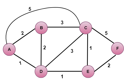
In the above figure, source vertex is A.

Step 1:

The first step is an initialization step. The currently known least cost path from A to its directly attached neighbors, B, C, D are 2,5,1 respectively. The cost from A to B is set to 2, from A to D is set to 1 and from A to C is set to 5. The cost from A to E and F are set to infinity as they are not directly linked to A.

Step	N	D(B),P(B)	D(C),P(C)	D(D),P(D)	D(E),P(E)	D(F),P(F)
1	A	2,A	5,A	1,A	∞	∞

Step 2:

In the above table, we observe that vertex D contains the least cost path in step 1. Therefore, it is added in N. Now, we need to determine a least-cost path through D vertex.

a) Calculating shortest path from A to B

v = B, w = D  

D(B) = min( D(B) , D(D) + c(D,B) )  

     = min( 2, 1+2)>  

     = min( 2, 3)  

The minimum value is 2. Therefore, the currently shortest path from A to B is 2.

b) Calculating shortest path from A to C

v = C, w = D  

D(B) = min( D(C) , D(D) + c(D,C) )  

     = min( 5, 1+3)  

     = min( 5, 4)  

The minimum value is 4. Therefore, the currently shortest path from A to C is 4.</p>

c) Calculating shortest path from A to E

v = E, w = D  

D(B) = min( D(E) , D(D) + c(D,E) )  

     = min( ∞,  1+1)  

     = min(∞, 2)  

The minimum value is 2. Therefore, the currently shortest path from A to E is 2.

Note: The vertex D has no direct link to vertex E. Therefore, the value of D(F) is infinity.

Step	N	D(B),P(B)	D(C),P(C)	D(D),P(D)	D(E),P(E)	D(F),P(F)
1	A	2,A	5,A	1,A	∞	∞
2	AD	2,A	4,D		2,D	∞

Step 3:

In the above table, we observe that both E and B have the least cost path in step 2. Let's consider the E vertex. Now, we determine the least cost path of remaining vertices through E.

a) Calculating the shortest path from A to B.

v = B, w = E  

D(B) = min( D(B) , D(E) + c(E,B) )  

     = min( 2 , 2+ ∞ )  

     = min( 2, ∞)  

The minimum value is 2. Therefore, the currently shortest path from A to B is 2.

b) Calculating the shortest path from A to C.

v = C, w = E  

D(B) = min( D(C) , D(E) + c(E,C) )  

     = min( 4 , 2+1 )  

     = min( 4,3)  

The minimum value is 3. Therefore, the currently shortest path from A to C is 3.

c) Calculating the shortest path from A to F.

v = F, w = E  

D(B) = min( D(F) , D(E) + c(E,F) )  

     = min( ∞ , 2+2 )  

     = min(∞ ,4)  

The minimum value is 4. Therefore, the currently shortest path from A to F is 4.

Step	N	D(B),P(B)	D(C),P(C)	D(D),P(D)	D(E),P(E)	D(F),P(F)
1	A	2,A	5,A	1,A	∞	∞
2	AD	2,A	4,D		2,D	∞
3	ADE	2,A	3,E			4,E

Step 4:

In the above table, we observe that B vertex has the least cost path in step 3. Therefore, it is added in N. Now, we determine the least cost path of remaining vertices through B.

a) Calculating the shortest path from A to C.

v = C, w = B  

D(B) = min( D(C) , D(B) + c(B,C) )  

     = min( 3 , 2+3 )  

     = min( 3,5)  

The minimum value is 3. Therefore, the currently shortest path from A to C is 3.

  

b) Calculating the shortest path from A to F.

v = F, w = B  

D(B) = min( D(F) , D(B) + c(B,F) )  

     = min( 4, ∞)  

     = min(4, ∞)  

The minimum value is 4. Therefore, the currently shortest path from A to F is 4.

Step	N	D(B),P(B)	D(C),P(C)	D(D),P(D)	D(E),P(E)	D(F),P(F)
1	A	2,A	5,A	1,A	∞	∞
2	AD	2,A	4,D		2,D	∞
3	ADE	2,A	3,E			4,E
4	ADEB		3,E			4,E

Step 5:

In the above table, we observe that C vertex has the least cost path in step 4. Therefore, it is added in N. Now, we determine the least cost path of remaining vertices through C.

a) Calculating the shortest path from A to F.

v = F, w = C  

D(B) = min( D(F) , D(C) + c(C,F) )  

     = min( 4, 3+5)  

     = min(4,8)  

The minimum value is 4. Therefore, the currently shortest path from A to F is 4.

Step	N	D(B),P(B)	D(C),P(C)	D(D),P(D)	D(E),P(E)	D(F),P(F)
1	A	2,A	5,A	1,A	∞	∞
2	AD	2,A	4,D		2,D	∞
3	ADE	2,A	3,E			4,E
4	ADEB		3,E			4,E
5	ADEBC					4,E

Final table:

Step	N	D(B),P(B)	D(C),P(C)	D(D),P(D)	D(E),P(E)	D(F),P(F)
1	A	2,A	5,A	1,A	∞	∞
2	AD	2,A	4,D		2,D	∞
3	ADE	2,A	3,E			4,E
4	ADEB		3,E			4,E
5	ADEBC					4,E
6	ADEBCF

Disadvantage:

Heavy traffic is created in Line state routing due to Flooding. Flooding can cause an infinite looping, this problem can be solved by using Time-to-leave field