Support vector machines

Introduction to SVM

Support vector machines (SVMs) are powerful yet flexible supervised machine learning algorithms which are used both for classification and regression. But generally, they are used in classification problems. In 1960s, SVMs were first introduced but later they got refined in 1990. SVMs have their unique way of implementation as compared to other machine learning algorithms. Lately, they are extremely popular because of their ability to handle multiple continuous and categorical variables.

Working of SVM

An SVM model is basically a representation of different classes in a hyperplane in multidimensional space. The hyperplane will be generated in an iterative manner by SVM so that the error can be minimized. The goal of SVM is to divide the datasets into classes to find a maximum marginal hyperplane (MMH).

The followings are important concepts in SVM −

• Support Vectors − Datapoints that are closest to the hyperplane is called support vectors. Separating line will be defined with the help of these data points.
• Hyperplane − As we can see in the above diagram, it is a decision plane or space which is divided between a set of objects having different classes.
• Margin − It may be defined as the gap between two lines on the closet data points of different classes. It can be calculated as the perpendicular distance from the line to the support vectors. Large margin is considered as a good margin and small margin is considered as a bad margin.

The main goal of SVM is to divide the datasets into classes to find a maximum marginal hyperplane (MMH) and it can be done in the following two steps −

• First, SVM will generate hyperplanes iteratively that segregates the classes in best way.
• Then, it will choose the hyperplane that separates the classes correctly. 

SVM Kernels

In practice, SVM algorithm is implemented with kernel that transforms an input data space into the required form. SVM uses a technique called the kernel trick in which kernel takes a low dimensional input space and transforms it into a higher dimensional space. In simple words, kernel converts non-separable problems into separable problems by adding more dimensions to it. It makes SVM more powerful, flexible and accurate. The following are some of the types of kernels used by SVM.

Linear Kernel: It can be used as a dot product between any two observations. The formula of linear kernel is as below −

K(x,xi)=sum(x∗xi)

From the above formula, we can see that the product between two vectors say 𝑥 & 𝑥𝑖 is the sum of the multiplication of each pair of input values.

Polynomial Kernel: It is more generalized form of linear kernel and distinguish curved or nonlinear input space. Following is the formula for polynomial kernel −

k(X,Xi)=1+sum(X∗Xi)^d

Here d is the degree of polynomial, which we need to specify manually in the learning algorithm.

Gaussian Kernel: It is used to perform transformation, when there is no prior knowledge about data.

Gaussian Kernel Formula

Hyperplane(Decision surface ):

For so long in this post we have been discussing the hyperplane, let’s justify its meaning before moving forward. The hyperplane is a function which is used to differentiate between features. In 2-D, the function used to classify between features is a line whereas, the function used to classify the features in a 3-D is called as a plane similarly the function which classifies the point in higher dimension is called as a hyperplane. Now since you know about the hyperplane lets move back to SVM.

Let’s say there are “m” dimensions:

thus the equation of the hyperplane in the ‘M’ dimension can be given as =

where,

Wi = vectors(W0,W1,W2,W3……Wm)

b = biased term (W0)

X = variables.

 

Properties of SVM

• Flexibility in choosing a similarity function
• Sparseness of solution when dealing with large data sets
• only support vectors are used to specify the separating hyperplane
• Ability to handle large feature spaces
• complexity does not depend on the dimensionality of the feature space
• Overfitting can be controlled by soft margin approach
• Nice math property: a simple convex optimization problem which is guaranteed to converge to a single global solution
• Feature Selection

 Disadvantages:

1. SVM algorithm is not suitable for large data sets.
2. SVM does not perform very well when the data set has more noise i.e. target classes are overlapping.
3. In cases where the number of features for each data point exceeds the number of training data samples, the SVM will underperform.
4. As the support vector classifier works by putting data points, above and below the classifying hyperplane there is no probabilistic explanation for the classification.

EM Algorithm

What is EM Algorithm ?

EM algorithm was proposed in 1997 by Arthur Dempster, Nan Laird, and Donald Rubin. It is basically used to find the local maximum likelihood parameters of a statistical model in case the latent variables are present or the data is missing or incomplete.

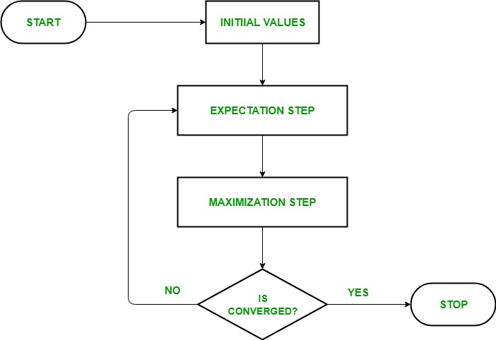
The EM Algorithm follows the following steps in order to find the relevant model parameters in the presence of latent variables.

1. Consider a set of starting parameters in incomplete data.

2. Expectation Step – This step is used to estimate the values of the missing values in the data. It involves the observed data to basically guess the values in the missing data.

3. Maximization Step – This step generates complete data after the Expectation step updates the missing values in the data.

4. Execute the step 2 and 3 until the convergence is met.

Convergence – The concept of convergence in probability is based on intuition. Let’s say we have two random variables if the probability of their difference is very small, it is said to be converged. In this case, convergence means if the values match each other.

How Does It Work?

The basic idea behind the EM algorithm is to use the observed data to estimate the missing data and then updating those values of the parameters. keeping the flowchart in mind, let us understand how the EM algorithm works.

1. In the starting stage, a set of initial parameters is considered. A set of unobserved and incomplete data is given to the system with an assumption that the observed data is coming from a specific model.
2. The next step is the Expectation Step or E-STEP. In this step, we use the observed data to estimate missing or incomplete data. It is basically used to update the variables.
3. The Maximization step or M-STEP is used to complete the data generated in the E-STEP. This step basically updates the hypothesis.
4. In the last step, it is checked whether the values are converging or not. If the values match, then we do nothing, else we will continue with step 2 and 3 until the convergence is met.

The EM algorithm is also known for clustering other than density estimation. So, let us try to understand the EM algorithm with the help of the Gaussian Mixture Model.

Gaussian Mixture Model

The GMM or Gaussian Mixture Model is a mixture model that uses a combination of probability distributions and also requires the estimation of mean and standard deviation parameters.

Even though there are a lot of techniques to estimate the parameters for a Gaussian Mixture Model, the most common technique is the Maximum Likelihood estimation.

Let us consider a case, where the data points are generated by two different processes and each process has a Gaussian probability distribution. But it is unclear, which distribution a given data point belongs to since the data is combined and distributions are similar. And the processes used for generating the data points represent the latent variables and influence the data. The EM algorithm seems like the best approach to estimate the parameters of the distributions.

In the EM algorithm, the E-STEP would estimate the expected value for each latent variable and the M-STEP would optimize the parameters of the distribution using the Maximum Likelihood.

Usage of EM algorithm –

• It can be used to fill the missing data in a sample.
• It can be used as the basis of unsupervised learning of clusters.
• It can be used for the purpose of estimating the parameters of Hidden Markov Model (HMM).
• It can be used for discovering the values of latent variables.

Advantages of EM algorithm –

• It is always guaranteed that likelihood will increase with each iteration.
• The E-step and M-step are often pretty easy for many problems in terms of implementation.
• Solutions to the M-steps often exist in the closed form.

Disadvantages of EM algorithm –

• It has slow convergence.
• It makes convergence to the local optima only.
• It requires both the probabilities, forward and backward (numerical optimization requires only forward probability).

Bayesian Belief Network

Bayesian belief network is key computer technology for dealing with probabilistic events and to solve a problem which has uncertainty. We can define a Bayesian network as:

"A Bayesian network is a probabilistic graphical model which represents a set of variables and their conditional dependencies using a directed acyclic graph."

It is also called a Bayes network, belief network, decision network, or Bayesian model.

Bayesian networks are probabilistic, because these networks are built from a probability distribution, and also use probability theory for prediction and anomaly detection.

Real world applications are probabilistic in nature, and to represent the relationship between multiple events, we need a Bayesian network. It can also be used in various tasks including prediction, anomaly detection, diagnostics, automated insight, reasoning, time series prediction, and decision making under uncertainty.

Bayesian Network can be used for building models from data and experts opinions, and it consists of two parts:

• Directed Acyclic Graph
• Table of conditional probabilities.

The generalized form of Bayesian network that represents and solve decision problems under uncertain knowledge is known as an Influence diagram.

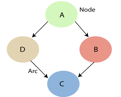
A Bayesian network graph is made up of nodes and Arcs (directed links), where:

• Each node corresponds to the random variables, and a variable can be continuous or discrete.
• Arc or directed arrows represent the causal relationship or conditional probabilities between random variables. These directed links or arrows connect the pair of nodes in the graph.
  These links represent that one node directly influence the other node, and if there is no directed link that means that nodes are independent with each other
  • In the above diagram, A, B, C, and D are random variables represented by the nodes of the network graph.
  • If we are considering node B, which is connected with node A by a directed arrow, then node A is called the parent of Node B.
  • Node C is independent of node A.

Note: The Bayesian network graph does not contain any cyclic graph. Hence, it is known as a directed acyclic graph or DAG.

The Bayesian network has mainly two components:

• Causal Component
• Actual numbers

Each node in the Bayesian network has condition probability distribution P(X_i |Parent(X_i) ), which determines the effect of the parent on that node.

Bayesian network is based on Joint probability distribution and conditional probability. So let's first understand the joint probability distribution:

Joint probability distribution:

If we have variables x1, x2, x3,....., xn, then the probabilities of a different combination of x1, x2, x3.. xn, are known as Joint probability distribution.

P[x₁, x₂, x₃,....., x_n], it can be written as the following way in terms of the joint probability distribution.

= P[x₁| x₂, x₃,....., x_n]P[x₂, x₃,....., x_n]

= P[x₁| x₂, x₃,....., x_n]P[x₂|x₃,....., x_n]....P[x_n-1|x_n]P[x_n].

In general for each variable Xi, we can write the equation as:

P(Xi|Xi-1,........., X1) = P(Xi |Parents(Xi ))

Explanation of Bayesian network:

Let's understand the Bayesian network through an example by creating a directed acyclic graph:

Example: Harry installed a new burglar alarm at his home to detect burglary. The alarm reliably responds at detecting a burglary but also responds for minor earthquakes. Harry has two neighbors David and Sophia, who have taken a responsibility to inform Harry at work when they hear the alarm. David always calls Harry when he hears the alarm, but sometimes he got confused with the phone ringing and calls at that time too. On the other hand, Sophia likes to listen to high music, so sometimes she misses to hear the alarm. Here we would like to compute the probability of Burglary Alarm.

Problem:

Calculate the probability that alarm has sounded, but there is neither a burglary, nor an earthquake occurred, and David and Sophia both called the Harry.

Solution:

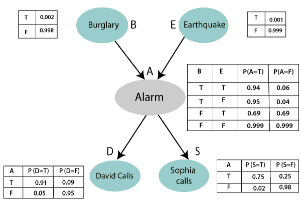
• The Bayesian network for the above problem is given below. The network structure is showing that burglary and earthquake is the parent node of the alarm and directly affecting the probability of alarm's going off, but David and Sophia's calls depend on alarm probability.
• The network is representing that our assumptions do not directly perceive the burglary and also do not notice the minor earthquake, and they also not confer before calling.
• The conditional distributions for each node are given as conditional probabilities table or CPT.
• Each row in the CPT must be sum to 1 because all the entries in the table represent an exhaustive set of cases for the variable.
• In CPT, a boolean variable with k boolean parents contains 2^K probabilities. Hence, if there are two parents, then CPT will contain 4 probability values

List of all events occurring in this network:

• Burglary (B)
• Earthquake(E)
• Alarm(A)
• David Calls(D)
• Sophia calls(S)

We can write the events of problem statement in the form of probability: P[D, S, A, B, E], can rewrite the above probability statement using joint probability distribution:

P[D, S, A, B, E]= P[D | S, A, B, E]. P[S, A, B, E]

=P[D | S, A, B, E]. P[S | A, B, E]. P[A, B, E]

= P [D| A]. P [ S| A, B, E]. P[ A, B, E]

= P[D | A]. P[ S | A]. P[A| B, E]. P[B, E]

= P[D | A ]. P[S | A]. P[A| B, E]. P[B |E]. P[E]

Let's take the observed probability for the Burglary and earthquake component:

P(B= True) = 0.002, which is the probability of burglary.

P(B= False)= 0.998, which is the probability of no burglary.

P(E= True)= 0.001, which is the probability of a minor earthquake

P(E= False)= 0.999, Which is the probability that an earthquake not occurred.

We can provide the conditional probabilities as per the below tables:

Conditional probability table for Alarm A:

The Conditional probability of Alarm A depends on Burglar and earthquake:

B	E	P(A= True)	P(A= False)
True	True	0.94	0.06
True	False	0.95	0.04
False	True	0.31	0.69
False	False	0.001	0.999

Conditional probability table for David Calls:

The Conditional probability of David that he will call depends on the probability of Alarm.

A	P(D= True)	P(D= False)
True	0.91	0.09
False	0.05	0.95

Conditional probability table for Sophia Calls:

The Conditional probability of Sophia that she calls is depending on its Parent Node "Alarm."

A	P(S= True)	P(S= False)
True	0.75	0.25
False	0.02	0.98

From the formula of joint distribution, we can write the problem statement in the form of probability distribution:

P(S, D, A, ¬B, ¬E) = P (S|A) *P (D|A)*P (A|¬B ^ ¬E) *P (¬B) *P (¬E).

= 0.75* 0.91* 0.001* 0.998*0.999

= 0.00068045.

Hence, a Bayesian network can answer any query about the domain by using Joint distribution.

The semantics of Bayesian Network:

There are two ways to understand the semantics of the Bayesian network, which is given below:

1. To understand the network as the representation of the Joint probability distribution.

It is helpful to understand how to construct the network.

2. To understand the network as an encoding of a collection of conditional independence statements.

It is helpful in designing inference procedure.

Ques.  Write a short note on Bayesian network.

 Or 

Explain the Bayesian network by taking an example . How is the Bayesian network representation for uncertainty knowledge ?

Answer:

• A Bayesian network is a probabilistic graphical model(PGM) which represents a set of variables and their conditional dependencies using a directed acyclic graph(DAG).
• These networks are built from a probability distribution, and also use probability theory for prediction and anomaly detection.
• Each  variable  is  associated  with  a  conditional  probability  table  which  gives  the probability  of  this  variable  for  different  values  of  the  variables  on  which  this  node depends.
• Using this model, it is possible to perform inference and learning.Bayesian  networks  that  model  a  sequence  of  variables  varying  in  time  are  called dynamic Bayesian networks
• Bayesian   networks   with   decision   nodes   which   solve  decision   problems   under uncertainly are Influence diagrams.

Explicit representation of conditional independencies Missing arcs encode conditional independence Efficient representation of joint PDF P(X) Generative model (not just discriminative): allows arbitrary queries to be answered, 

e.g. P (lung cancer=yes | smoking=no, positive X-ray=yes ) = ?

For example, a Bayesian network could represent the probabilistic relationships between diseases and symptoms. Given symptoms, the network can be used to compute the probabilities of the presence of various diseases. Efficient algorithms can perform inference and learning in Bayesian networks.

Another Example:

Applications:

• Prediction
• Anomaly detection
• Diagnostics
• Automated insight
• Reasoning
• Time series prediction
• Decision making under uncertainty.

 

 

Ques. Explain the role of  prior probability and posterior probability in bayesian classification. 

Answer:

Prior Probability:

Bayesian statistical inference is the probability of an event before new data is collected.This is the best rational assessment of the probability of an outcome based on current knowledge.

It shows the likelihood of an outcome in a given dataset.

For example,

In the Mortgage case, P(Y) is the default rate on a home mortgage, which is 2%. P(Y|X) is called the conditional probability, which provides the probability of an outcome given the evidence, that is, when the value of X is known.

Posterior Probability:

It is calculated using Bayes’ Theorem.Prior probability gets updated when new data is available,to produce a more accurate measure of a potential outcome.

A posterior probability can subsequently become a prior for a new updated posterior probability as new information arises and is incorporated into the analysis.

Ques. Explain the method of handling approximate inference in Bayesian networks.

Answer:

Inference over a Bayesian network can come in two forms. The first is simply evaluating the joint probability of a particular assignment of values for each variable (or a subset) in the network

In exact inference, we analytically compute the conditional probability distribution over the variables of interest.

Methods of handling approximate inference in Bayesian Networks:

Simulation Methods:

It uses the network to generate samples from the conditional probability distribution and estimate conditional probabilities of interest when the number of samples is sufficiently large.

With machine learning, the inputs are known exactly, but the model is unknown prior to training. Regarding output, the differences are more subtle. Both give an output, but the source of uncertainty is different.

Variational Methods:

Variational Bayesian methods are a family of techniques for approximating intractable integrals arising in Bayesian inference and machine learning.