B-Trees

B - Trees ( Balanced Search Trees ) 

B-trees differ significantly from red-black trees in that B-tree nodes may have many children, from a handful to thousands. That is, the "branching factor" of a B-tree can be quite large, although it is usually determined by the characteristics of the disk unit used. B-trees are similar to red-black trees in that every n-node B-tree has height O(lg n), although the height of a B-tree can be considerably less than that of a red-black tree because its branching factor can be much larger. Therefore, B-trees can also be used to implement many dynamic-set operations in time O(lg n).

A B-tree is a tree data structure that keeps data sorted and allows searches, insertions, and deletions in logarithmic amortized time. Unlike self-balancing binary search trees, it is optimized for systems that read and write large blocks of data. It is most commonly used in database and file systems.

Properties 

A B-tree T is a rooted tree (with root root[T]) having the following properties.

1. Every node x has the following fields:

    a. n[x], the number of keys currently stored in node x,

    b. the n[x] keys themselves, stored in nondecreasing order: key₁[x]≤key₂[x]≤.............key_n[x][x], and

    c. leaf [x], a boolean value that is TRUE if x is a leaf and FALSE if x is an internal node.

2. If x is an internal node, it also contains n[x] + 1 pointers c₁ [x], c₂[x], . . . , c_n[x]+1[x] to its children. Leaf nodes have no children, so their c_i fields are undefined.

3. The keys key_i[x] separate the ranges of keys stored in each subtree: if k_i is any key stored in the subtree with root c_i[x], then

k₁ ≤ key₁[x] ≤ k₂ ≤ key₂[x] ≤..........key_n[x][x] ≤ k_n[x]+1 .

4. Every leaf has the same depth, which is the tree's height h.

5. There are lower and upper bounds on the number of keys a node can contain. These bounds can be expressed in terms of a fixed integer t >= 2 called the minimum degree of the B-tree:

    a. Every node other than the root must have at least t - 1 keys. Every internal node other than the root thus has at least t children. If the tree is nonempty, the root must have at least one key.

    b. Every node can contain at most 2t - 1 keys. Therefore, an internal node can have at most 2t children. We say that a node is full if it contains exactly 2t - 1 keys.

The simplest B-tree occurs when t = 2. Every internal node then has either 2, 3, or 4 children, and we have a 2-3-4 tree. In practice, however, much larger values of t are typically used.

Properties of a B-tree (of order M)

1. All data is stored in leaves, in a sorted order.
2. The root is a leaf or has between 2 and M children
3. Each interior node is at least half full -- has between éM/2ù and M children
4. All leaves are at the same depth
5. All leaves are at least half full -- store between éL/2ù and L data items

Height of a B tree

Basic operations on B-Trees 

Searching a B-tree

Searching a B-tree is much like searching a binary search tree, except that instead of making a binary, or "two-way," branching decision at each node, we make a multiway branching decision according to the number of the node's children. More precisely, at each internal node x, we make an (n[x] + 1)-way branching decision.

B-TREE-SEARCH is a straightforward generalization of the TREE-SEARCH procedure defined for binary search trees. B-TREE-SEARCH takes as input a pointer to the root node x of a subtree and a key k to be searched for in that subtree. The top-level call is thus of the form B-TREE-SEARCH(root[T], k). If k is in the B-tree, B-TREE-SEARCH returns the ordered pair (y,i) consisting of a node y and an index i such that key_i[y] = k. Otherwise, the value NIL is returned.

B-TREE-SEARCH(x, k)

1  i = 1
2  while i ≤ n[x] and k ≥ keyi[x]
3       do i = i + 1
4  if i ≤ n[x] and k = keyi[x]
5      then return (x, i)
6  if leaf [x]
7      then return NIL
8      else DISK-READ(ci[x])
9           return B-TREE-SEARCH(ci[x], k)

B-Tree create

To build a B-tree T, we first use B-TREE-CREATE to create an empty root node and then call B-TREE-INSERT to add new keys. Both of these procedures use an auxiliary procedure ALLOCATE-NODE, which allocates one disk page to be used as a new node in O(1) time. We can assume that a node created by ALLOCATE-NODE requires no DISK-READ, since there is as yet no useful information stored on the disk for that node.

B-TREE-CREATE(T)

1  x = ALLOCATE-NODE()
2  leaf[x] = TRUE
3  n[x] = 0
4  DISK-WRITE(x)
5  root[T] = x

B-TREE-CREATE requires O(1) disk operations and O(1) CPU time.

Splitting a node with t = 4. Node y is split into two nodes, y and z, and the median key S of y is moved up into y's parent.

B-Tree  Insert 

Insertion:

At the leaf node level, insertions are made. The following algorithm must be followed to place an item into B Tree.

1. Navigate the B Tree until you find the suitable leaf node to insert the node.
2. If there are fewer than m-1 keys in the leaf node, insert the element in ascending order.
3. Else, it should proceed to the next step if the leaf node contains m-1 keys.
1. In the rising sequence of elements, add the new element.
2. In the middle, divide the node into two nodes.
3. The median element should be pushed up to its parent node.
4. If the parent node has the same m-1 number of keys as the child node, split it.

Figure: Splitting the root with t = 4. Root node r is split in two, and a new root node s is created. The new root contains the median key of r and has the two halves of r as children. The B-tree grows in height by one when the root is split.

B-TREE-INSERT(T,k)

1  r = root[T]
2  if n[r] = 2t - 1
3      then s = ALLOCATE-NODE()
4           root[T] = s
5           leaf[s] = FALSE
6           n[s] = 0
7           c1[s] = r
8           B-TREE-SPLIT-CHILD(s,1,r)
9           B-TREE-INSERT-NONFULL(s,k)
10  else B-TREE-INSERT-NONFULL(r,k)

Lines 3-9 handle the case in which the root node r is full: the root is split and a new node s (having two children) becomes the root. Splitting the root is the only way to increase the height of a B-tree. Figure spliting illustrates this case. Unlike a binary search tree, a B-tree increases in height at the top instead of at the bottom. The procedure finishes by calling B-TREE-INSERT-NONFULL to perform the insertion of key k in the tree rooted at the nonfull root node. B-TREE-INSERT-NONFULL recurses as necessary down the tree, at all times guaranteeing that the node to which it recurses is not full by calling B-TREE-SPLIT-CHILD as necessary.

The auxiliary recursive procedure B-TREE-INSERT-NONFULL inserts key k into node x, which is assumed to be nonfull when the procedure is called. The operation of B-TREE-INSERT and the recursive operation of B-TREE-INSERT-NONFULL guarantee that this assumption is true.

B-TREE-INSERT-NONFULL(x,k)

1  i = n[x]
2  if leaf[x]
3      then while i ≥ 1 and k < keyi[x]
4               do keyi+1 [x] = keyi[x]
5                  i = i - 1
6           keyi+1[x] = k
7           n[x] = n[x] + 1
8           DISK-WRITE(x)
9  else while i ≥ 1 and k < keyi[x]
10               do i = i - 1
11       i = i + 1
12       DISK-READ(ci[x])
13       if n[ci[x]] = 2t - 1
14          then B-TREE-SPLIT-CHILD(x,i,ci[x])
15               if k > keyi[x]
16                  then i = i + 1
17       B-TREE-INSERT-NONFULL(ci[x],k)

The B-TREE-INSERT-NONFULL procedure works as follows. Lines 3-8 handle the case in which x is a leaf node by inserting key k into x. If x is not a leaf node, then we must insert k into the appropriate leaf node in the subtree rooted at internal node x. In this case, lines 9-11 determine the child of x to which the recursion descends. Line 13 detects whether the recursion would descend to a full child, in which case line 14 uses B-TREE-SPLIT-CHILD to split that child into two nonfull children, and lines 15-16 determine which of the two children is now the correct one to descend to. (Note that there is no need for a DISK-READ(c_i[x]) after line 16 increments i, since the recursion will descend in this case to a child that was just created by B-TREE-SPLIT-CHILD.) The net effect of lines 13-16 is thus to guarantee that the procedure never recurses to a full node. Line 17 then recurses to insert k into the appropriate subtree. 

Example: 

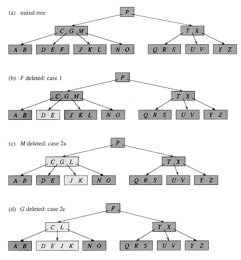
 B-Tree  Deletion 

At the leaf nodes, deletion is also conducted. It can be a leaf node or an inside node that must be destroyed. To delete a node from a B tree, use the following algorithm.

1. Find the position of the leaf node.
2. If the leaf node has more than m/2 keys, delete the required key from the node.
3. If the leaf node lacks m/2 keys, fill in the gaps with the eighth or left sibling element.
1. If the left sibling has more than m/2 elements, shift the intervening element down to the node where the key is deleted and push the largest element up to its parent.
2. If the right sibling has more than m/2 items, shift the intervening element down to the node where the key is deleted and push the smallest element up to the parent.
4. Create a new leaf node by merging two leaf nodes and the parent node's intervening element if neither sibling has more than m/2 elements.
5. If the parent has less than m/2 nodes, repeat the operation on the parent as well.

If the node to be destroyed is an internal node, its in-order successor or predecessor should be used instead. Because the successor or predecessor will always be on the leaf node, the operation will be similar to deleting the node from the leaf node.

Example: 

                                                 source: staff.ustc.edu.cn

Applications

• Because accessing values held in a vast database saved on a disc is a very time-consuming activity, the B tree is used to index the data and enable fast access to the actual data stored on the discs.
• In the worst situation, searching an unindexed and unsorted database with n key values takes O(n) time. In the worst-case scenario, if we use B Tree to index this database, it will be searched in O(log n) time.
• A B-tree, in particular:
  • keeps keys sorted for sequential traversal and uses a hierarchical index to reduce disc reads
  • insertions and deletions are sped up by using partially filled blocks.
  • a recursive algorithm that keeps the index balanced
     

 

Some solved question 

Create B-tree of order 5 from the following lists of data items: 20, 30, 35, 85, 10, 55, 60, 25, 5, 65, 70, 75, 15, 40, 50, 80, 45.