Suppose, We are given a sequence (chain) (A1, A2……An) of n matrices to be multiplied, and we wish to compute the product (A1A2…..An). We can evaluate the above expression using the standard algorithm for multiplying pairs of matrices as a subroutine once we have parenthesized it to resolve all ambiguities in how the matrices are multiplied together. Matrix multiplication is associative, and so all parenthesizations yield the same product. For example, if the chain of matrices is (A1, A2, A3, A4) then we can fully parenthesize the product (A1A2A3A4) in five distinct ways:
1:-(A1(A2(A3A4))) ,
2:-(A1((A2A3)A4)),
3:- ((A1A2)(A3A4)),
4:-((A1(A2A3))A4),
5:-(((A1A2)A3)A4) .
We can multiply two matrices A and B only if they are compatible. the number of columns of A must equal the number of rows of B. If A is a p x q matrix and B is a q x r matrix, the resulting matrix C is a p x r matrix. The time to compute C is dominated by the number of scalar multiplications is pqr. we shall express costs in terms of the number of scalar multiplications.For example, if we have three matrices (A1,A2,A3) and its cost is (10x100),(100x5),(5x500) respectively. so we can calculate the cost of scalar multiplication is 10*100*5=5000 if ((A1A2)A3), 10*5*500=25000 if (A1(A2A3)), and so on cost calculation. Note that in the matrix-chain multiplication problem, we are not actually multiplying matrices. Our goal is only to determine an order for multiplying matrices that has the lowest cost. That is here is minimum cost is 5000 for the above example. So the problem is we can perform many times of cost multiplications and repeatedly the calculation is performed. so this general method is very time-consuming and tedious. So we can apply dynamic programming to solve this kind of problem.
when we use the Dynamic programming technique we shall follow some steps.
- Characterize the structure of an optimal solution.
- Recursively define the value of an optimal solution.
- Compute the value of an optimal solution.
- Construct an optimal solution from computed information.
we have matrices of any order. our goal is to find the optimal cost multiplication of matrices. when we solve this kind of problem using DP step 2 we can get
m[i , j] = min { m[i , k] + m[i+k , j] + pi-1*pk*pj } if i < j…. where p is dimension of matrix , i ≤ k < j …..
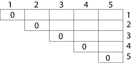
Example: We are given the sequence {4, 10, 3, 12, 20, and 7}. The matrices have size 4 x 10, 10 x 3, 3 x 12, 12 x 20, 20 x 7. We need to compute M [i,j], 0 ≤ i, j≤ 5. We know M [i, i] = 0 for all i.
Let us proceed with working away from the diagonal. We compute the optimal solution for the product of 2 matrices.
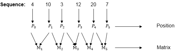
Here P0 to P5 are Position and M1 to M5 are matrix of size (pi to pi-1)
On the basis of sequence, we make a formula
In Dynamic Programming, initialization of every method done by '0'.So we initialize it by '0'.It will sort out diagonally.
We have to sort out all the combination but the minimum output combination is taken into consideration.
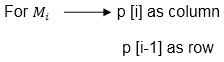
Calculation of Product of 2 matrices:
1. m (1,2) = m1  x m2
           = 4 x 10 x  10 x 3
           = 4 x 10 x 3 = 120

2. m (2, 3) = m2 x m3
            = 10 x 3  x  3 x 12
            = 10 x 3 x 12 = 360

3. m (3, 4) = m3 x m4
            = 3 x 12  x  12 x 20
            = 3 x 12 x 20 = 720

4. m (4,5) = m4 x m5
           = 12 x 20  x  20 x 7
           = 12 x 20 x 7 = 1680
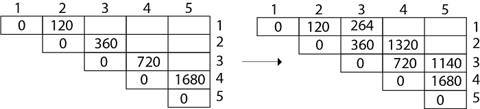
- We initialize the diagonal element with equal i,j value with '0'.
- After that second diagonal is sorted out and we get all the values corresponded to it
Now the third diagonal will be solved out in the same way.
Now product of 3 matrices:
M [1, 3] = M1 M2 M3- There are two cases by which we can solve this multiplication: ( M1 x M2) + M3, M1+ (M2x M3)
- After solving both cases we choose the case in which minimum output is there.

M [1, 3] =264
As Comparing both output 264 is minimum in both cases so we insert 264 in table and ( M1 x M2) + M3 this combination is chosen for the output making.
M [2, 4] = M2 M3 M4- There are two cases by which we can solve this multiplication: (M2x M3)+M4, M2+(M3 x M4)
- After solving both cases we choose the case in which minimum output is there.

M [2, 4] = 1320
As Comparing both output 1320 is minimum in both cases so we insert 1320 in table and M2+(M3 x M4) this combination is chosen for the output making.
M [3, 5] = M3 M4 M5- There are two cases by which we can solve this multiplication: ( M3 x M4) + M5, M3+ ( M4xM5)
- After solving both cases we choose the case in which minimum output is there.

M [3, 5] = 1140As Comparing both output 1140 is minimum in both cases so we insert 1140 in table and ( M3 x M4) + M5this combination is chosen for the output making.
Now Product of 4 matrices:
M [1, 4] = M1 M2 M3 M4There are three cases by which we can solve this multiplication:
- ( M1 x M2 x M3) M4
- M1 x(M2 x M3 x M4)
- (M1 xM2) x ( M3 x M4)
After solving these cases we choose the case in which minimum output is there
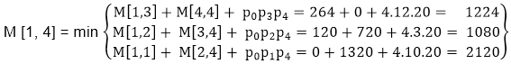
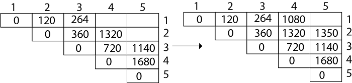
M [1, 4] =1080
As comparing the output of different cases then '1080' is minimum output, so we insert 1080 in the table and (M1 xM2) x (M3 x M4) combination is taken out in output making,
M [2, 5] = M2 M3 M4 M5There are three cases by which we can solve this multiplication:
- (M2 x M3 x M4)x M5
- M2 x( M3 x M4 x M5)
- (M2 x M3)x ( M4 x M5)
After solving these cases we choose the case in which minimum output is there
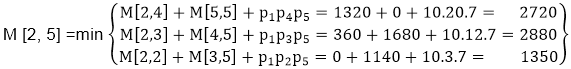
M [2, 5] = 1350As comparing the output of different cases then '1350' is minimum output, so we insert 1350 in the table and M2 x( M3 x M4 xM5)combination is taken out in output making.
Now Product of 5 matrices:
M [1, 5] = M1 M2 M3 M4 M5There are five cases by which we can solve this multiplication:
- (M1 x M2 xM3 x M4 )x M5
- M1 x( M2 xM3 x M4 xM5)
- (M1 x M2 xM3)x M4 xM5
- M1 x M2x(M3 x M4 xM5)
After solving these cases we choose the case in which minimum output is there
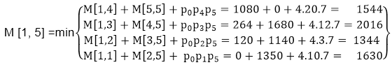
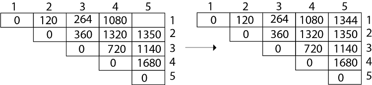
M [1, 5] = 1344As comparing the output of different cases then '1344' is minimum output, so we insert 1344 in the table and M1 x M2 x(M3 x M4 x M5)combination is taken out in output making.
Final Output is:
Step 3: Computing Optimal Costs: let us assume that matrix Ai has dimension pi-1x pi for i=1, 2, 3....n. The input is a sequence (p0,p1,......pn) where length [p] = n+1. The procedure uses an auxiliary table m [1....n, 1.....n] for storing m [i, j] costs an auxiliary table s [1.....n, 1.....n] that record which index of k achieved the optimal costs in computing m [i, j].
The algorithm first computes m [i, j] ← 0 for i=1, 2, 3.....n, the minimum costs for the chain of length 1.
Algorithm of Matrix Chain Multiplication

We will use tables to construct an optimal solution.
Step 1: Constructing an Optimal Solution:

Analysis: There are three nested loops. Each loop executes a maximum n times.
- l, length, O (n) iterations.
- i, start, O (n) iterations.
- k, split point, O (n) iterations
Body of loop constant complexity
Total Complexity is: O (n3)
Algorithm with Explained Example
Question: P [7, 1, 5, 4, 2}
Solution: Here, P is the array of a dimension of matrices.
So here we will have 4 matrices:
A17x1  A21x5  A35x4  A44x2
i.e.
First Matrix A1 have dimension 7 x 1
Second Matrix A2 have dimension 1 x 5
Third Matrix A3 have dimension 5 x 4
Fourth Matrix A4 have dimension 4 x 2

Let say,
From P = {7,	1,	5,	4,	2} - (Given)
And P is the Position
p0 = 7,	p1 =1,	p2 = 5,	p3 = 4,	p4=2.
Length of array P = number of elements in P
∴length (p)= 5
From step 3
Follow the steps in Algorithm in Sequence
According to Step 1 of Algorithm Matrix-Chain-Order
Step 1:
n ← length [p]-1
Where n is the total number of elements
And length [p] = 5
∴ n = 5 - 1 = 4
n = 4
Now we construct two tables m and s.
Table m has dimension [1.....n, 1.......n]
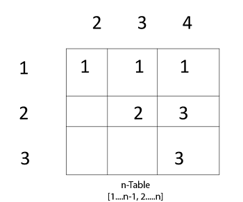
Table s has dimension [1.....n-1, 2.......n]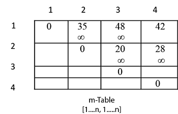
Now, according to step 2 of Algorithm
for i ← 1 to n
this means: for i ← 1 to 4 (because n =4)
for  i=1
m [i, i]=0
m [1, 1]=0
Similarly for i = 2, 3, 4
m [2, 2] = m [3,3] = m [4,4] = 0
i.e. fill all the diagonal entries "0" in the table m
Now,
l ← 2 to n
l ← 2 to 4    (because n =4 )
Case 1:
1. When l - 2
 for (i ← 1 to n - l + 1)
	    i ← 1 to 4 - 2 + 1
	    i ← 1 to 3

When i = 1
  do   j ← i + l - 1
	         j ← 1 + 2 - 1
	         j ← 2
     i.e. j = 2
Now, m [i, j] ← ∞
	i.e. m [1,2] ← ∞
Put ∞ in m [1, 2] table
	  for k ← i to j-1
	       k ← 1 to 2 - 1
	       k ← 1 to 1
            k = 1
Now q ← m [i, k] + m [k + 1, j] + pi-1 pk pj
			for l = 2
			     i = 1
			     j =2
			    k = 1
	    q ← m [1,1] + m [2,2] + p0x p1x p2
             and m [1,1] = 0
		  for i ← 1 to 4
     ∴ q ← 0 + 0 + 7 x 1 x 5
	    q ← 35
We have m [i, j] = m [1, 2] = ∞
Comparing q with m [1, 2]
		q < m [i, j]
		i.e. 35 < m [1, 2]
		35 < ∞
		True
	then, m [1, 2 ] ← 35  (∴ m [i,j] ← q)
		s [1, 2] ← k
	and the value of k = 1
		s [1,2 ] ← 1
Insert "1" at dimension s [1, 2] in table s. And 35 at m [1, 2]
2. l remains 2
L = 2
		    i ← 1 to n - l + 1
		    i ← 1 to 4 - 2 + 1
		    i ← 1 to 3
		for i = 1 done before
		Now value of i becomes 2
		i = 2
j ←  i + l - 1
		 j ←  2 + 2 - 1
		 j ←  3
		j = 3
m [i , j]  ← ∞
i.e. m [2,3] ← ∞
	Initially insert ∞ at m [2, 3]
Now, for k ← i to j - 1
		k ← 2 to 3 - 1
		k ← 2 to 2
		i.e. k =2
		Now, q ← m [i, k] + m [k + 1, j] + pi-1 pk pj
		For l =2
			     i = 2
			     j = 3
			     k = 2
		q ← m [2, 2] + m [3, 3] + p1x p2 x p3
		              q ← 0 + 0 + 1 x 5 x 4
					  q ← 20
					  Compare q with m [i ,j ]
		If q < m [i,j]
	i.e. 20 < m [2, 3]
20 < ∞
True
Then m [i,j ] ← q
	     m [2, 3 ] ← 20
and s [2, 3] ← k
	and k = 2
s [2,3] ← 2
3. Now i become 3
 i = 3
  l = 2
j ← i + l - 1
j ← 3 + 2 - 1
j ← 4
j = 4
Now, m [i, j ] ← ∞
          m [3,4 ] ← ∞
Insert ∞ at m [3, 4]
  for k ← i to j - 1
	       k ← 3 to 4 - 1
	       k ← 3 to 3
	i.e. k = 3
Now, q ← m [i, k] + m [k + 1, j] + pi-1 pk pj
i = 3
				l = 2
				j = 4
				k = 3
q ← m [3, 3] + m [4,4] + p2  x p3 x p4
q ← 0 + 0 + 5 x 2 x 4
q   40
Compare q with m [i, j]
		If q < m [i, j]
		   40 < m [3, 4]
		   40 < ∞
		True
Then, m [i,j] ← q
	      m [3,4] ← 40
and s [3,4] ← k
	  s [3,4] ← 3
Case 2: l becomes 3
      L = 3
	      for i = 1 to n - l + 1
	           i = 1 to 4 - 3 + 1
		 i = 1 to 2
When i = 1
	j ← i + l - 1
	j ← 1 + 3 - 1
         j ← 3
	j = 3
Now, m [i,j]   ← ∞
          m [1, 3]  ←  ∞
for k ← i to j - 1
     k ← 1 to 3 - 1
     k ← 1 to 2
Now we compare the value for both k=1 and k = 2. A minimum of two will be placed in m [i,j] or s [i,j] respectively.
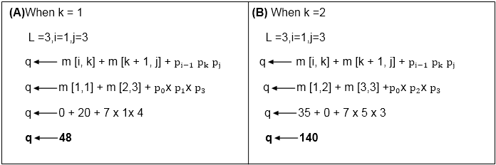
Now from above
Value of q become minimum for k=1
		∴ m [i,j] ← q
		    m [1,3] ← 48
Also m [i,j] > q
i.e. 48 < ∞
∴ m [i , j] ← q
   m [i, j] ← 48
and s [i,j] ← k
i.e. m [1,3] ← 48
	  s [1, 3] ←  1
Now i become 2
	i = 2
	 l = 3
then j ← i + l -1
	   j ←  2 + 3 - 1
	   j ← 4
	   j = 4
	   so m [i,j] ← ∞
m [2,4] ← ∞
Insert initially ∞ at m [2, 4]
      for k   ← i to j-1
	      k  ← 2 to 4 - 1
	      k  ← 2 to 3
Here, also find the minimum value of m [i,j] for two values of k = 2 and k =3
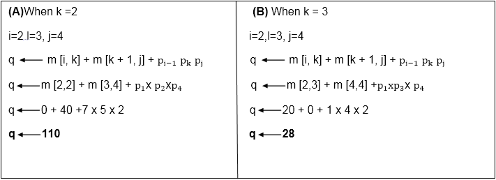
But 28 <     ∞
 So m [i,j] ← q
    And q  ← 28
m [2, 4]  ← 28
and   s [2, 4]  ← 3
e. It means in s table at s [2,4] insert 3 and at m [2,4] insert 28.
Case 3: l becomes 4
L = 4
	   For i ← 1 to n-l + 1
		i ← 1 to 4 - 4 + 1
		i ← 1
		i = 1
	do j  ← i + l - 1
	     j ← 1 + 4 - 1
	     j ← 4
	    j = 4
Now m [i,j]  ←  ∞
        m [1,4] ←  ∞
for k  ← i to j -1
     k ← 1 to 4 - 1
     k  ← 1 to 3
When k = 1
q  ←  m [i, k] + m [k + 1, j] + pi-1 pk pj
q  ← m [1,1] + m [2,4] + p0xp4x p1
q ← 0 + 28 + 7 x 2 x 1
q  ← 42
Compare q and m [i, j]
m [i,j] was ∞
i.e. m [1,4]
if q < m [1,4]
   42< ∞
    True
Then m [i,j] ← q
	m [1,4] ← 42
and s [1,4]  1	? k =1
When k = 2
	L = 4, i=1, j = 4
q ← m [i, k] + m [k + 1, j] + pi-1 pk pj
q ← m [1, 2] + m [3,4] + p0 xp2 xp4
q ← 35 + 40 + 7 x 5 x 2
q  ← 145
Compare q and m [i,j]
Now m [i, j]
      i.e. m [1,4] contains 42.
So if q < m [1, 4]
But 145 less than or not equal to m [1, 4]
   So 145 less than or not equal to 42.
So no change occurs.
When k = 3
	l = 4
	i = 1
	j = 4
q  ←  m [i, k] + m [k + 1, j] + pi-1 pk pj
q ← m [1, 3] + m [4,4] + p0 xp3 x p4
q ← 48 + 0 + 7 x 4 x 2
q  ← 114
Again q less than or not equal to m [i, j]
	i.e. 114 less than or not equal to m [1, 4]
	       114 less than or not equal to 42
So no change occurs. So the value of m [1, 4] remains 42. And value of s [1, 4] = 1
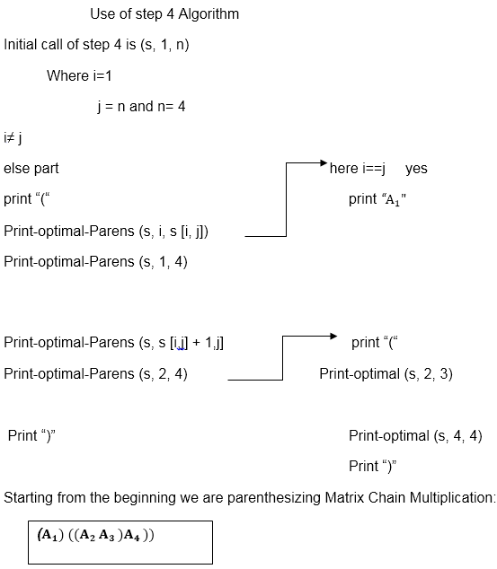
Now we will make use of only s table to get an optimal solution.
Matrix multiplication
Matrix multiplication is an important operation in many mathematical and image-processing applications. Suppose we want to multiply two matrices A and B, each of size n x n, multiplication is operation is defined as
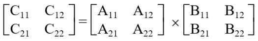
C11 = A11 B11 + A12 B21
C12 = A11 B12 + A12 B22
C21 = A21 B11 + A22 B21
C22 = A21 B12 + A22 B22
This approach is very costly as it required 8 multiplications and 4 additions.
Algorithm
Complexity Analysis
The innermost statement is enclosed within three for loops. That statement runs in constant time, i.e. in O(1) time. Running time of algorithm would be,
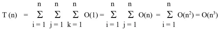
Running time of this algorithm is cubic, i.e. O(n3)
Matrix Multiplication using Strassen’s Method
Strassen suggested a divide and conquer strategy-based matrix multiplication technique that requires fewer multiplications than the traditional method. The multiplication operation is defined as follows using Strassen’s method:
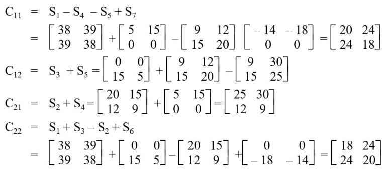
C11 = S1 + S4 – S5 + S7
C12 = S3 + S5
C21 = S2 + S4
C22 = S1 + S3 – S2 + S6
Where,
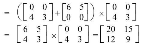
S1 = (A11 + A22) * (B11 + B22)
S2 = (A21 + A22) * B11
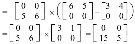
S3 = A11 * (B12 – B22)
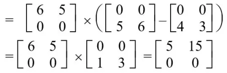
S4 = A22 * (B21 – B11)
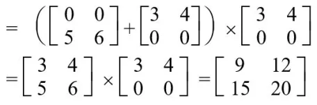
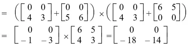
S5 = (A11 + A12) * B22
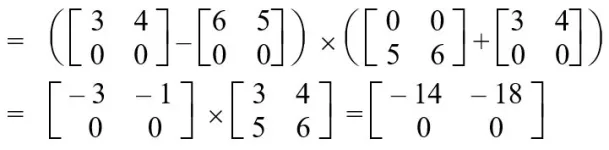
S6 = (A21 – A11) * (B11 + B12)
S7 = (A12 – A22) * (B21 + B22)
Let us check if it is same as the conventional approach.
C12 = S3 + S5
= A11 * (B12 – B22) + (A11 + A12) * B22
= A11 * B12 – A11 * B22 + A11 * B22 + A12 * B22
= A11 * B12 + A12 * B22
This is same as C12 derived using conventional approach. Similarly we can derive all Cij for strassen’s matrix multiplication.
Algorithm
Complexity Analysis of Matrix Multiplication using Divide and Conquer approach
The conventional approach performs eight multiplications to multiply two matrices of size 2 x 2. Whereas Strassen’s approach performs seven multiplications on the problem of size 1 x 1, which in turn finds the multiplication of 2 x 2 matrices using addition. In short, to solve the problem of size n, Strassen’s approach creates seven problems of size (n – 2). Recurrence equation for Strassen’s approach is given as,
T(n) = 7.T(n/2)
Two matrices of size 1 x 1 needs only one multiplication, so the base case would be, T (1) = 1. Let us find the solution using the iterative approach. By substituting n = (n / 2) in above equation,
T(n/2) = 7.T(n/4)
⇒ T(n) = 72.T(n/22)
.
.
.
T(n) = 7k.T(2k)
Let’s assume n = 2k ⇒ k = log2 n
T (n) = 7k .T(2k/2k)
= 7k .T (1)
= 7k
= 7log2 n
= nlog2 7
= n2.81 < n3
Thus, running time of Strassen’s matrix multiplication algorithm O(n2.81), which is less than cubic order of traditional approach. The difference between running time becomes significant when n is large.
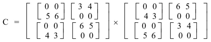
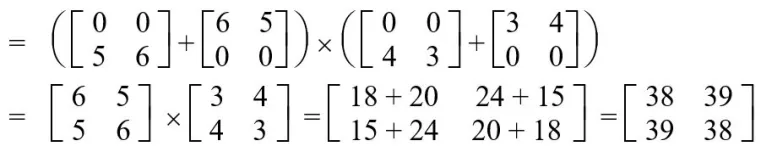
Example of Matrix Multiplication using Divide and Conquer Approach
Problem: Multiply given two matrices A and B using Strassen’s approach, where
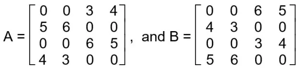
Solution:
let,
S1 = (A11 + A22) x (B11 + B22)
S2 = (A21 + A22) x B11
S3 = A11 x (B12 – B22)
S4 = A22 x (B21 – B11)
S5 = (A11 + A12) x B22
S6 = (A11 – A11) x (B11 + B12)
S7 = (A12 – A22) x (B21 + B22)


No comments:
Post a Comment