AI BMC 021 Unit-3

Propositional Logic

Propositional logic is a branch of logic that deals with propositions, which are statements that can be either true or false. It makes complex expressions by using logical connectives like AND, OR, NOT, and IMPLIES, and then applies rules to determine their truth values.

Propositional Logic in Artificial Intelligence

Artificial intelligence (AI) uses propositional logic as one of the major methods of knowledge representation using logical propositions. Propositions are statements that are either true or false but not both. More complex expressions are created by combining statements with logical operators like AND, OR, NOT, and IMPLIES. This enables an AI system to make better decisions using logical reasoning.

Artificial intelligence applies propositional logic in rule-based reasoning, automated theorem proving, and expert system decision-making. In machine learning, inference rules like Modus Ponens and Resolution allow machines to draw conclusions on the basis of the facts provided.

Propositions, in artificial intelligence, are sentences that are considered to state facts, situations, or claims about the world to enable the logical reasoning of the machines. The propositional logic expression consists of symbols (for these truths) and logical operators, often represented with parenthesis.

Example

Following are few examples of propositions (declarative statements) −

• The sun rises in the east.
• A triangle has four sides. (False)
• Water boils at 100C under normal atmospheric pressure.
• 2 + 2 = 5. (False)
• A self-driving car can operate without human intervention.

Facts about Propositional logic

Propositional logic is a formal system applied in mathematics, computer science, and artificial intelligence for reasoning about logical statements.

• It pays no attention to the context and content, it just determines whether propositions are true or false based on their structure.
• In propositional logic, operations are ordered according to precedence: Negation (¬) leads to conjunction (), then disjunction (), implication (→), and biconditional ().
• Truth tables are applied to determine whether a logical expression is valid, satisfiable, or equivalent.
• Propositional logic is limited because it can't express a relationship between the objects and quantifiers like "for all" or "there exists," where these are handled by First Order Logic.
• A proposition must be a declarative statement that holds a truth value of true or false, like the sky is blue. Statements like "Where is Krish?" is not a proposition because it is not declarative statement.

Key Components of Propositional Logic

Propositional logic involves basic building blocks such as propositions, logical connectives, and truth tables to form logical expressions which simplifies knowledge representation that help AI to reason and make decisions based on facts.

Propositions (Statements)

Propositional logic deals with two kinds of propositions, atomic and compound propositions which form the base for logical expressions.

• Atomic proposition: An atomic proposition is an basic statement which cannot be split into smaller units. It has a single proposition sign.

  For example, statement like "The car is parked in the garage".
• Compound Proposition: A compound proposition is formed by combining two or more atomic propositions using logical connectives like AND, OR, NOT, Implies.For example, "She likes coffee OR she likes tea".

Logical Connectives

Logical connectives, also known as logical operators, are symbols that connect or alter propositions in propositional logic. They help to form complex propositions and determine the relationships between the components. Below are the main types −

Conjunction

The combination of two propositions is only true if both of the propositions are true.

Example

The sun is shining AND it is a warm day.

• P = The sun is shining.
• Q = It is a warm day. → P Q.

The combination of above two statements become P Q. The statement, ("The sun is shining AND it is a warm day") is TRUE only if both the statements is true, if either P or Q is FALSE the entire statement is FALSE.

Disjunction (OR, )

The disjunction of two propositions is true if at least one of the propositions is true.

Example

"It is raining OR it is snowing." True if either condition is true, or both.

• P = It is raining.
• Q = It is snowing. → P Q.

Negation (NOT, ¬)

The negation of a proposition reverses its truth value, if the proposition is true, the negation is false, and vice versa.

For example, "The car is NOT parked in the driveway."(True if the car is not parked in the driveway.)

Implication (IF-THEN, →)

An implication says that if the first proposition is true, then the second has to be true as well. It is only false when the first statement is right and the second statement is wrong. It is sometimes called if-then rules.

For example, "If it rains, then the ground gets wet." (False only if it rains and the ground does not get wet.)

Biconditional (IF AND ONLY IF, )

A biconditional statement is true whenever the two propositions have the same truth value-both true or both false.

For example, "She is happy IF AND ONLY IF she passed the exam." (True only if she passed the exam and is happy, or neither of them is true.)

Table for Propositional Logic Connectives

The following table presents the fundamental connectives used in Propositional Logic, along with their symbols, meanings, and examples −

Connective Symbols	Words	Terms	Example
	AND	Conjunction	A B
	OR	Disjunction	A B
→	Implies	Implication	A → B
	If and only if	Biconditional	A B
	either A or B but not both	Exclusive Or	A B
¬ or ~	NOT	Negation	¬A or ~B

Truth Table

A truth table is a systematic representation of all possible truth values of propositions and their logical combinations in propositional logic, particularly in artificial intelligence.

It helps to determine the validity of logical statements by showing how the truth value of a compound proposition changes with respect to the truth values of its individual components.

Conjunction

The AND operation of P Q is true if both the propositional variable P and Q are true.

The truth table is as follows −

P	Q	P Q
True	True	True
True	False	False
False	True	False
False	False	False

Disjunction

The OR operation of two Propositional variable P Q is true if atleast any of the propositional variable p or q is true.

The truth table is as follows −

P	Q	P Q
True	True	True
True	False	True
False	True	True
False	False	False

Implication

An implication P → Qrepresents if P then Q. It is false if P is true and Q is false. The rest cases are true.

The truth table is as follows −

P	Q	P → Q
True	True	True
True	False	False
False	True	True
False	False	True

Bi-conditional

P Q is Bi-conditional if both P and Q have both truth value i.e, both are false or both are true.

The truth table is as follows −

P	Q	P Q
True	True	True
True	False	False
False	True	False
False	False	True

Exclusive OR

P Q is said to be exclusive OR if exactly one of the propositions is true but not both.

The truth table is as follows −

P	Q	P Q
True	True	False
True	False	True
False	True	True
False	False	False

Negation

The logical operation which reverses the truth value of a proposition. For example if P is true the negation of P is false, and vice versa.

The truth table is as follows −

P	¬P
True	False
False	True

Tautologies, Contradictions, and Contingencies

Tautologies: A tautology is a proposition that is true regardless of the truth values assigned to its component propositions. In other words, no matter what we assign to the components of this statement, the final result will always be true.

Example: P ¬P (P OR NOT P) is always true since either P is true or P is false, which means that one part of the OR conditions is always true.

Contradiction: A contradiction is a proposition that is always wrong, no matter which truth values are assigned to its components. It represents a statement that simply cannot be true.

Example: P ¬P (P AND NOT P) is always false because P cannot be simultaneously true and false.

Contingency: A contingency is a proposition that may not be necessarily true or false. The truth value of the entire statement is determined by the truth value of the propositions. That is, it may be true in some situations but false in others.

Example: P Q (P AND Q) is true if both P and Q are true, but false otherwise.

Precedence of connectives

In propositional logic, the order of operations (precedence) is as follows −

Precedence	Operators
First preference	Parenthesis
Second preference	Negation
Third preference	Conjunction(AND)
Fourth preference	Disjunction(OR)
Fifth preference	Implication
Sixth preference	Biconditional

Note: Operators with the same precedence are evaluated from left to right.

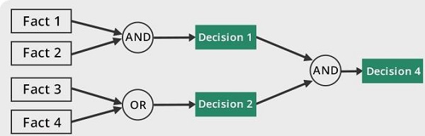
Example: Shopping Decision

Statement: "If the item is on sale AND I have a coupon, I will buy it OR I will wait for a better deal."

Propositions: A proposition is a declarative statement that might be true or false, but not both.

• P = The item is on sale.
• Q = I have a coupon.
• R = I will buy it.
• S = I will wait for a better deal.

Propositional Logic Expression: A propositional logic expression is the set of propositions joined together by logical connectives to form a meaningful statement. We write the logical expression using symbols and connectives.

(P Q) → (R S)

Step-by-Step Evaluation −

Here we follow the logical reasoning step by step.

• Conjunction: Evaluate (P Q) and see whether the two conditions that have to be satisfied, sale and coupon, are met.
• Disjunction: Consider (R S ) to determine whether the decision is to buy or wait.
• Implication: If P and Q are true, then the conclusion must be R or S, so the AI system will make the right decision.

This is how we implement the precedence rules in propositional logic, first evaluating the parentheses, then conjunction, followed by disjunction, and finally implication (IF-THEN) to reach a logical decision.

Logical equivalence

Logical equivalence in propositional logic means that two statements, or propositions, always have the same truth value regardless of the truth values assigned to the individual components.

• Symbols: "" or "" represents logical equivalence. P Q means "P is logically equivalent to Q".
• It simplifies complex logical phrases, which makes the AI system understand and interpret more effectively.
• Logical equivalence lets AI draw new conclusions from preceding knowledge. If two propositions are true and the AI knows one is true, then it can conclude that the other proposition is also true.
• In some AI systems like expert systems, uses logical equivalence to reduce the complexity of search or reasoning by replacing complex phrases with simpler, equivalent phrases.

Properties of Operators

Commutation: The order of variables in AND () and OR () does not affect the result. ( swapping positions doesnt change meaning.). Following are examples of commutation.

• P Q Q P
• P Q Q P

Association: The way propositions are grouped in AND () and OR () does not matter. ((Parentheses can be rearranged without changing meaning.). Following are examples of association.

• (P Q) R P (Q R)
• (P Q) R P (Q R)

Distribution: AND () can be distributed over OR (), and OR () can be distributed over AND (). ((Like multiplying over addition in algebra.). Following are examples of distribution.

• P (Q R) (P Q) (P R)
• P (Q R) (P Q) (P R)

De Morgan's Law: Describes how negation interacts with both conjunction and disjunction. Following are examples of De Morgan's Law.

• ¬(P Q) ¬P ¬Q
• ¬(P Q) ¬P ¬Q

Double Negation: A negation of a negation is the same proposition. Following are examples of double negation.

• ¬(¬P)P

Implication (→): Implication can be rewritten using NOT (¬) and OR (). Following are examples of Implication.

• P → Q ¬P Q

Idempotence: An operation is idempotent if repeating it a number of times yields the same result as doing it once. Following are examples of Idempotence.

• P P P
• P P P

Syntax of Propositional Logic

The syntax of propositional logic specifies rules and symbols required to construct valid logical propositions. It consists of propositions, logical connectives, and parentheses that assist in representing knowledge in a structured way.

• Propositions (Atomic Statements): These are simple statements that may be either true or false. They are usually represented by capital letters like P, Q, R, etc.
• Logical Connectives (Operators): The symbols that can be used to connect or transform propositions in a way that combines or alters their truth values such as , , ¬, →,
• Parentheses: are used to group propositions and order operations properly e.g, (P Q) → R
• Compound Propositions: It is a logical statement which is obtained by combining several atomic propositions through logical connectives like , , ¬, →, and . For example, (P Q) (¬R).

Applications of Propositional Logic in AI

Following are the applications of propositional logic −

• Automated Reasoning: Automated reasoning uses propositional logic which enables machine to deduce new knowledge from existing facts. This helps in problem-solving and decision making.

• For example, let the known facts be "The room is dark" and "The lights turn on". If AI detects darkness, it automatically turn on lights. This way it can use or infer the existing knowledge.

• Knowledge Representation: AI uses propositional logic to represent facts and relationships using propositions (statements that are either true or false) and logical connectivities such as , , ¬ and →. This logical representation helps AI to make decisions and answer queries quicker by simplifying complex representation into a structured form.

• For example, let the statements be "The customer buys a smartphone." and "The system recommends a phone case". The logical representation for this would be P → Q meaning if the customer buys a smartphone, the AI system will recommend to buy a phone case.

• Decision Making: AI uses propositional logic to make decisions based on conditions.

• For example, "If the car is low on fuel (P), and the fuel station is nearby (Q), then the car will stop for refueling" (P Q → Refuel).

• Planning and problem-solving: These are fundamental activities of AI, where machines process a situation, establish objectives, and decide a sequence of steps to achieve a desired outcome. Propositional logic helps the AI describe goals, constraints, and conditions in a structured way, so that systems can logically determine what actions to take next.

• For example, "If a meeting room is available (P) and all the participants are free (Q), the AI schedules the meeting" (P Q) → R.

• Expert System: Expert Systems uses propositional logic to represent facts and apply rule-based reasoning to draw conclusions.

• For example, "The applicant has a stable job (P) , The applicant has a good credit score (Q), The loan is approved" (P Q) → R here we use logical representation to draw conclusions.

• Game Playing: In games like chess, AI uses propositional logic to make decisions.

• For example, ""If the queen is near the king (P) and we can block it (Q), then we will move the piece" (P Q → Move Piece).

• Natural Language Processing: Propositional logic enables AI to evaluate language patterns, extract meaning, and make logical conclusions in chatbots, virtual assistants, machine translation, and automated text processing.
• For example, for the sentence "If it rains (P), take an umbrella (Q)", the AI learns that if it is raining, it should take an umbrella.

Limitations of Propositional Logic

Following are the limitations of propositional logic

• Propositional logic handles declarative statements as true or false however it can't show objects and how they relate to each other. For example, "The sun is hot" propositional logic only tells whether this statement is true or false, but it cannot tell the relationship between sun and other objects like cloud.
• It can't express ideas like "All humans are mortal" or "Some students passed the exam" because it doesn't have universal () or existential () quantifiers.
• We can't represent complex statements with variables such as "If a person is a student then they have an ID card."
• As the number of facts increases propositional logic, requires too many individual propositions, making it inefficient for large AI systems.
• It struggles with incomplete or uncertain data, which many real-world AI applications need.
• Since propositional logic has these drawbacks, we use First-Order Logic (FOL) to overcome them. FOL adds objects, relationships, and quantifiers, increasing its usefulness for AI reasoning.

Predicate Logic

Propositional logic deals with declarative statements that are either true or false. However, it has a significant disadvantage it cannot state relationships between objects or convey general statements quickly.

For example, consider the following sentence. "The sky is hot" propositional logic only decides that a statement is true or false, but it cannot explain the relationship between the sun and heat. Similarly, if we want to declare that "All students in a class like mathematics," propositional logic would require a different statement for each student, which is impractical for huge collections of things.

This is where First-Order Logic comes in. FOL expands propositional logic by including quantifiers and variables, allowing us to construct such assertions more efficiently.

First-Order Logic in Artificial intelligence

First-Order Logic, more popularly known as Predicate Logic, or First-Order Predicate Logic for short, is an extension of Propositional Logic. Unlike propositional logic which only tells that a statement is either true or false, First-Order Logic allows us to define relationship between objects, general rules, and quantified statements.

Key components of First-Order Logic

The fundamental components of First-Order Logic (FOL), which helps in the systematic representation of relationships, objects, and logical propositions, are as follows −

• Constants are different objects or constant values that exist inside given domain. For example − Krish, Bob, 5, Apple.
• Variables are symbols that can take several values inside a particular domain. Commonly used symbols for variables are x,y,z. If the domain consists of students, then x could represent any student in the class.
• Predicates are statements that describe properties of objects or their relationships. They accept at least one parameter, which may be a constant or a variable. For example − Father(John, Robert). Here father is predicate which tells the relation between John and Robert.
• Functions map elements to distinct values. They take arguments in the form of input elements and return a single value as output. For example − Age(Alice) = 25 → means "Alice's age is 25."
• Quantifiers tell whether a sentence is true for all objects in the domain or just one. For example − xLikes(x,Math) → "All students like Mathematics." and xLikes(x,Math) → "There exists at least one student who likes Mathematics."
• Logical connectives enable to logically combine numerous statements or propositions. They allow complicated statements to be constructed from simpler ones. For example − CompletesTraining(x)→EligibleForPromotion(x). If an employee x completes the required training, then they automatically become eligible for a promotion.

Logical Components in Formal Logic

The following table lists the constants, variables, functions, predicates, quantifiers, and logical connectives which are used to build formal logic −

Components	Examples
Constants	1, 5, Apple, Bob, India
Variables	x, y, z, a, b
Predicates	Father, Teacher, Brother
Functions	sqrt, LeftLegOf, AgeOf, add(x, y)
Quantifiers	∀ (for all), ∃ (there exists)
Connectives	∧ (and), ∨ (or), ¬ (not), → (implies), ↔ (if and only if)

Syntax and Semantics of First-Order Logic (FOL)

The syntax of FOL describes the form of valid assertions by employing constants, variables, predicates, functions, quantifiers, and logical connectives. Statements are composed of words (which represent objects) and atomic formulae (which convey facts).

The semantics of first-order logic (FOL) define the meaning of assertions by interpreting predicates and words throughout a domain. An interpretation gives real-world meaning to objects and relationships.

Example

The following example demonstrates how syntax and semantics are applied in First-Order Logic (FOL) to represent a real-world statement −

• Consider a statement "Every customer who makes a purchase receives an invoice".
• The FOL representation of the statement using syntax and semantics is as follows x(Customer(x)Purchases(x,Product)→ReceivesInvoice(x))
• Thus, syntax defines the structure, and semantics give it meaning.

Quantifiers in First-Order Logic

Quantifiers in First-Order Logic define the number of objects in the domain that meet a specific condition. They allow us to communicate statements about all or some objects in a systematic manner.

Types of Quantifiers in FOL

First-Order Logic has two main types of quantifiers −

• Universal Quantifier ( ) "For All"
• Existential Quantifier ( ) "There Exists"

Universal Quantifier ( ): The universal quantifier (x) is used to state that a statement applies to all items in the domain. It is used to convey general truths or rules.

For example, let the statement be "All employees in a company must follow the rules." By using FOL the representation would be x(Employee(x)→FollowsRules(x)) meaning "For every x, if x is an employee, then x follows the rules."

Existential Quantifier ( ): The existential quantifier "x" indicates that at least one object in the domain meets the provided condition.It is used to indicate that something exists without listing all instances.

For example, let the statement be "There is at least one employee who received a promotion. The FOL representation would be "x(Employee(x)ReceivedPromotion(x)) meaning "There exists some x, such that x is an employee and x received a promotion."

Sentences in First-Order Logic

In First-Order Logic (FOL), sentences are used to represent facts and relationships. These sentences can be classified into atomic sentences and complex sentences, as explained below −

Atomic Sentences

An atomic sentence is the most basic form of a statement in First-Order Logic. It consists of a predicate and arguments, which can be either constants or variables. An atomic statement asserts a fact about things without using logical connectives.

Structure of Atomic Sentences: Predicate(Argument 1,Argument 2,...,Argument n)

where −

• The predicate represents a property or relationship.
• The arguments represent objects (constants or variables).

Example

The following example demonstrate the use of atomic sentences in First-Order Logic to represent facts and relationships −

• Teacher(John, Mathematics) This atomic sentence states that John is a teacher of Mathematics.

Complex sentence

Two or more atomic statements connected by logical connectives like AND (), OR (), NOT (¬), Implies (→), and Bi-conditional () create a complex sentence. These sentences allow us to express more complex logical statements.

Example

The following examples demonstrate the use of complex sentences in First-Order Logic to represent facts and relationships −

• (y Teacher(y) Teaches(y, Math)) "There exists at least one teacher who teaches Mathematics."
• (x Customer(x) → Buys(x, TutorialsPointCourses)) "For all customers, if x is a customer, then x buys courses from Tutorials Point."
• (y Employee(y) WorksFor(y, TutorialsPoint)) "There exists at least one employee who works for Tutorials Point."

Free and Bound Variables in First-Order Logic

Variables in FOL can be either free or bounded depending on the fact that a variable is controlled by any quantifier.

Free Variable

A free variable cannot be quantified using or . It can hold any value but has no fixed meaning unless assigned.

Example

Let us consider a statement "y is the price of a product."

• The FOL representation for the above statement will be P(y) (where P(y) means y is the price of a product).
• Here, y is free because we don't specify which products price we are referring to.

Bound Variable

A bound variable is within the scope of a quantifier and is dependent on it, so its value is limited by the quantifier.

Example

Let the sentence be "There exists a product whose price is less than $10."

• The FOL representation of the above sentence is yP(y) (where P(y) means y is less than $10).
• Here, the existential quantifier () constrains the variable y, indicating that it is applicable to a specific product in the context.

Challenges and limitations of First Order Logic

When utilizing First-Order Logic (FOL) for knowledge representation and reasoning, several key challenges and limitations arise, as follows −

• Challenges in Handling Uncertainty: FOL requires facts to be definitively true or false, making it difficult to represent probabilistic or uncertain information.
• High Computational Demands: When dealing with extensive knowledge bases, logical inference in FOL can become slow and resource-intensive.
• Limited Expressive Power: Concepts from the real world that involve fuzzy or probabilistic logic, such as "most people" or "approximately," are difficult for FOL to articulate.
• Rigid Rule-Based Framework: The necessity for facts and rules to be explicitly defined results in a structure that is inflexible and struggles to incorporate new information.
• Common-Sense thinking Difficulty: FOL finds it difficult to manage common sense thinking that incorporates assumptions, exceptions, or insufficient information.

Inference in First-Order Logic

Inference in First-Order Logic (FOL) involves deriving new facts or statements from existing ones. This process is crucial for reasoning, knowledge representation, and automating logical deductions. Before we delve into some inference rules, let's first cover some fundamental concepts of FOL.

Substitution

Substitution is a fundamental operation in first-order logic that involves replacing a variable with a specific constant or phrase within an expression. This process is essential for effectively applying inference rules.

• When we write F[b/y], we are substituting the variable y with the constant b in the formula F.
• Using quantifiers for substitution needs to be done carefully to maintain logical consistency.
• First-Order Logic enables reasoning about specific objects and entire categories within a given domain.

Equality

In first-order logic (FOL), equality is an important aspect that allows us to express that two terms refer to the same object. The equality operator (=) is used to confirm that two expressions point to the same entity.

• The expression ¬(a = b) indicates that a and b are not identical objects.

For example, the statement Manager(Alex) = Sophia means that Sophia is the manager of Alex. Combining negation with equality helps to show that two concepts are distinct.

FOL Inference Rules for Quantifier

The inference rules for FOL are an extension of Propositional Logic by adding quantifiers and predicates. The rules below are the key ones:

Universal Generalization

Universal generalization is a valid inference rule that asserts if premise P(c) holds true for any arbitrary element c within the universe of discourse, we can conclude that x P(x) is also true.

If premise P(c) holds true for any arbitrary element c in the discourse universe we can arrive at the conclusion that x P(x).

It can be represented as − P(c), x P(x)

• Universal Generalization (UG )is valid only if c represents a general case applicable to all elements in the domain.

Example

Let us say the given statement is like this Loves(John, IceCream), Loves(Mary, IceCream), Loves(Sam, IceCream) the FOL representation using inference rule is as below −

• x Loves(x, IceCream) (if John, Mary, and Sam represent all entities).

Universal Instantiation

Universal Instantiation (UI) is an inference rule for First-Order Logic that derives a particular instance from a universally quantified statement. If it is true for all items of a domain, then it has to be the case for any specific element in the domain as well.

According to the UI rule, we can infer any sentence P(c) by replacing every object in the discourse universe with a ground term c (a constant within domain x) from x P(x).

It can be represented as − x P(x), P(c)

• According to the UI rule, any sentence P(c) is derivable, replacing a ground word c-for any object belonging to the universe of discourse-as a ground substitution for any x P(x).
• UI enables thinking of individual circumstances from universal facts.
• This is widely applied in theorem proving and automated reasoning.
• UI is the negation of Universal Generalization (UG).

Example

Let us say the given statement be "Everyone who teaches at a university has an advanced degree." x(Teaches(x,University)→ HasAdvancedDegree(x)) [ x P(x)].

• By applying Universal Instantiation (UI) inference rule we can infer that for a specific professor, say Dr. Amrit − Teaches(Dr.Amrit,University)→ HasAdvancedDegree(Dr.Amrit).

Existential Instantiation

Existential Instantiation (EI) is a First-Order Logic inference rule that allows for the replacement of an existentially quantified variable with a new, arbitrary constant in order to represent an unknown but existing entity.

This rule indicates that from the formula x P(x), one can deduce P(c) by introducing a new constant symbol c.

It can be represented as − x P(x), P(c)

• EI is also known as Existential Elimination.

• It can only be used once to replace an existential sentence with a particular instance.

• The new knowledge base (KB) is not logically equal to the old KB; yet, if the old KB was satisfactory, the new one is still satisfactory.

• According to EI, we can infer P(c) from xP(x) by introducing a new constant c.

• The inserted constant c must be new and not previously used in the KB.

Example

Let us say the given statement is "Someone has published a research paper." x (HasPublishedResearch(x)) [ x P(x) ].

• By applying the Existential Instantiation (EI) inference rule, we can infer that for a specific researcher, say Dr. Arjun − HasPublishedResearch(Dr.Arjun).

Existential Introduction

Existential Introduction (EI), often referred to as Existential Generalization (EG), is a valid inference rule in First-Order Logic. It allows us to introduce an existential quantifier when we can confirm that a proposition holds true for at least one instance.

It can be represented as − P(c), x P(x)

• It lets us move from a specific instance to a more general existential statement.

• If P(c) is true for a certain c, we can infer that there exists some x for which P(x) is true.

• The new existential statement is logically valid but different from the statement in question.

Example

Let us say the given statement is "Mr. Raj works at Tutorials Point." WorksAt(Mr.Raj, TutorialsPoint) [ P(c) ].

• By applying the Existential Introduction (EI) inference rule, we can generalize that "There exists someone who works at Tutorials Point." − x (WorksAt(x, TutorialsPoint)).

Generalized Modus Ponens (GMP) Rule

Generalized Modus Ponens is an extension of the traditional Modus Ponens rule of First-Order Logic. It allows multiple premises, variables, and substitutions. This facilitates logical reasoning by substituting variables in the premises and making replacements to reach conclusions.

Generalized Modus Ponens can be described as "P implies Q and P is asserted to be true, therefore Q must be true.

It can be represented as − P1→Q1,P2→Q2,,Pn→Qn,P1P2Pn, Q1Q2Qn

• Combines three steps of natural deduction (Universal Elimination, And Introduction, Modus Ponens) into one.

• Provides direction and simplification to the proof process for standard inferences.

Example

Let us say the given rule is "If a person works at Tutorials Point and has expertise in AI, then they are an AI Instructor." x (WorksAt(x, TutorialsPoint) HasExpertise(x, AI) → AIInstructor(x))

• Given facts: WorksAt(Ravi, TutorialsPoint)

• HasExpertise(Ravi, AI): By applying the Generalized Modus Ponens (GMP) inference rule, we can conclude: AIInstructor(Ravi).

What is Resolution

Resolution is a logical method that is used to validate statements by showing that assuming the negation leads to a contradiction. Essentially, it assesses the truth of a claim by presuming it is false and then proving that this assumption is impossible.

What is Resolution in First-Order Logic

A resolution is a rule in first-order logic (FOL) that allows us to derive new conclusions from previously established data. According to the concept of proof by contradiction, if assuming something is incorrect results in a contradiction, the assumption must be true.

The resolution approach is widely employed in logic-based problem solving and automated reasoning because it produces systematic, thorough, and efficient proofs of logical statements.

Why Do We Use Resolution

Resolution is commonly used in various fields of artificial intelligence and automated reasoning. Here are some key reasons for choosing resolution −

• Prove Statements Logically Resolution uses contradiction to assess if a statement is true or false.

• Automate Logical Reasoning - Allows computers to automatically draw conclusions from provided facts.

• Solve Problems in AI and Logic Programming - Used in Prolog and other AI applications for rule-based reasoning.

• Ensure Consistency in Knowledge-Based Systems - Assists in detecting inconsistencies and maintaining valid information.

• Verify Software and Systems - Ensures that software, security protocols, and hardware are working properly.

Key Components in Resolution

Resolution in First-Order Logic (FOL) depends on several key components that enhance the effectiveness of the inference process. They are −

Clause

A clause is a dis-junction that serves as a fundamental unit in resolution-based proofs. Following are the examples to better understand the Clauses −

• P(x)¬Q(x) → This expression consists of two literals linked by OR ().

• ¬ABC → This expression includes three literals, meaning at least one of them must be true.

Literals

A literal is either the atomic proposition (fact) or its negation. Literals are the building blocks of clauses. Here is an example of literals.

• P(x) is a positive literal that is either true or false.

• ¬Q(y) is a negative literal which is the negation of a fact.

Unification

Unification is the operation of two logical expressions by determining the correct substitutions for the variables to make both expressions equal. Here is an example of Unification.

• Let us consider two predicates − Predicate 1: Loves (x, Mary).

• Predicate 2: Loves (John,y).

To unify these two predicates, we have to find the substitutes for x and y such that they become identical. Substituting x=John and y=Mary gives us Loves(John, Mary). So, after unification, both predicates are the same.

Substitution

Substitution is the replacement of variables by definite values or words in a logical formulation for more specific expression. It is used in unification, resolution, and inference rules to make logical assertions more specific. Below is the example of substitution −

• Consider this predicate with a function: Teaches(Prof, Subject). Substituting = {Prof/Dr. Smith, Subject/Mathematics} yields the results in Teaches(Dr. Smith, Mathematics).

Skolemization

Skolemization is the process of removing existential quantifiers () by introducing Skolem functions or constants.

• Let us consider a statement, x y Loves(x, y), which means "for every x, there exists some y such that x loves y."

• To remove y, we introduce a Skolem function f(x), resulting in x Loves(x, f(x)), where f(x) represents a specific person that x loves, making the statement fully quantifier-free.

Steps for Resolution in First-Order Logic (FOL)

The resolution process involves systematically modifying logical statements and utilizing unification and resolution principles to either derive a contradiction or establish the desired outcome. Below are the key steps involved in FOL resolution −

• Convert statements to First-Order Logic (FOL) and express the given information using FOL notation.

• Convert FOL sentences into Clausal Form (CNF) by removing implications, moving negations inward, standardizing variables, applying Skolemization, and converting to conjunctive normal form.

• Negate the assertion to be verified - Assume the negation of the goal and include it in the list of clauses.

• Apply Unification: Find relevant variable substitutions to make literals identical.

• Use the Resolution Rule: Identify complementing literals and resolve them to create new clauses.

• Repeat until a contradiction or proof is found. Resolve until an empty clause () is derived (contradiction) or the goal statement is proven.

Example for Resolution in First-Order Logic

Let us consider the following statements −

• Every employee of Tutorials Point is knowledgeable.

• John is an employee of Tutorials Point.

• Prove that John is knowledgeable.

Step1: Convert statements to First-Order Logic (FOL)

• Statement 1: x (Employee(x, TutorialsPoint) → Knowledgeable(x))

• Statement 2: Employee(John, TutorialsPoint)

• Statement to Prove: Knowledgeable(John)

Step2: Convert FOL sentences into Clausal Form (CNF)

Remove Implications:

• ¬Employee(x, TutorialsPoint) Knowledgeable(x)

• Employee(John, TutorialsPoint)

Step3: Negate the Assertion to be Verified

To apply proof by contradiction, we assume the negation of the goal statement and add it to the set of clauses.

• Negated Goal: ¬Knowledgeable(John)

Step4: Apply Unification

Unification is performed to match variables and make expressions identical, allowing further resolution.

• Unify: x = John in Clause 1

• Substituting in Clause 1: ¬ Employee(John, TutorialsPoint) Knowledgeable(John)

Step5: Use the Resolution Rule

Resolution is applied to eliminate complementary literals and derive a new clause.

• Resolving Clause 2 (Employee(John, TutorialsPoint)) with Clause 1 (¬Employee(John, TutorialsPoint) Knowledgeable(John))

• Employee(John, TutorialsPoint) and ¬Employee(John, TutorialsPoint) cancel out.

• New Clause: Knowledgeable(John)

• The new clause Knowledgeable(John) is derived, bringing us closer to proving the goal.

Step6: Repeat Until a Contradiction or Proof is Found

The final resolution step confirms the goal by contradiction. Resolving Clause 3 (¬Knowledgeable(John)) with Knowledgeable(John). The literals cancel out, resulting in an empty clause ({}).

• Since an empty clause is derived, it confirms that the original goal (Knowledgeable(John)) is true.

Examples of Resolution in AI

Resolution plays a crucial role in various AI applications as it enables automated reasoning and logical inferences. Here are some key examples of how resolution is applied in AI.

• AI has an impact on Automated Theorem Proving - Resolution to prove mathematical theorems without human intervention. Programs like the Lean Theorem Prover and the Coq Proof Assistant use Resolution to check mathematical proofs.

• Expert Systems - AI systems use rule-based reasoning to draw logical conclusions. In medical diagnosis, expert systems like MYCIN use resolution to guess diseases based on symptoms and patient information.

• Natural Language Processing (NLP) - Resolution helps to break down and show meaning. AI-based NLP models such as IBM Watson and Google's BERT, apply resolution methods to find logical connections between words and boost language understanding.

Limitations of Resolution

Below are some key limitations of the resolution method in logical inference

• Computational Complexity: It produces numerous intermediate clauses, making it slow when dealing with large knowledge bases.

• Lack of Expressiveness: Transforming to CNF limits the expressiveness of some logical propositions.

• Handling Infinite Domains: There are challenges with recursive definitions and infinite problem sets.

Example 1 — Simple propositional / predicate implication

Sentence:

1. (P -> Q) and P

Step 1 — eliminate implication

• P -> Q becomes (not P) or Q.
  So the sentence is: ((not P) or Q) and P

Step 2 — negation movement

• No negation to push in further.

Step 3 — variables

• No variables.

Step 4 — prenex / quantifiers

• None.

Step 5 — skolemize

• None.

Step 6 — drop universals

• None.

Step 7 — CNF

• Already: ((not P) or Q) and P

Step 8 — clauses (as sets of literals)

• Clause1: {not P, Q}

• Clause2: {P}

Example 2 — Universal implication (classic)

Sentence:
2) For all x, if Human(x) then Mortal(x). And Human(Socrates).

Write:

• For all x (Human(x) -> Mortal(x))

• Human(Socrates)

Step 1 — eliminate implication

• Human(x) -> Mortal(x) becomes (not Human(x)) or Mortal(x).

Step 2 — move negations

• No negation over quantifiers except inside literal not Human(x).

Step 3 — standardize variables

• Only x used once; OK.

Step 4 — prenex

• Already: forall x (not Human(x) or Mortal(x))

Step 5 — skolemize

• No existentials, so nothing to skolemize.

Step 6 — drop universal

• Drop "forall": not Human(x) or Mortal(x).

Step 7 — CNF

• Already in CNF.

Step 8 — clauses

• Clause1: {not Human(x), Mortal(x)}

• Clause2: {Human(Socrates)}

Example 3 — Existential quantifier

Sentence:
3) There exists someone whom John loves.
Write: Exists x Loves(John, x)

Step 1 — eliminate implication

• None.

Step 2 — move negation

• None.

Step 3 — standardize variables

• Only x present; OK.

Step 4 — prenex

• Exists x Loves(John, x)

Step 5 — skolemize

• Replace existential x by a Skolem constant a (since it does not depend on universal variables).
  So becomes: Loves(John, a)

Step 6 — drop universals

• None.

Step 7 — CNF

• Already a single atomic formula, which is a clause.

Step 8 — clauses

• Clause1: {Loves(John, a)}

(Here "a" is a new Skolem constant representing some person John loves.)

Example 4 — Universal existence (Skolem function)

Sentence:
4) For every person x, there exists a mother y of x such that Parent(y, x) and Female(y).
Write: For all x, Exists y (Parent(y, x) and Female(y))

This needs a Skolem function because the existence depends on x.

Step 1 — eliminate implication

• None.

Step 2 — push negation

• None.

Step 3 — standardize variables

• x, y unique; fine.

Step 4 — prenex

• For all x Exists y (Parent(y, x) and Female(y))

Step 5 — skolemize

• Replace Exists y by a Skolem function m(x) (a mother function dependent on x).
  So formula becomes: For all x (Parent(m(x), x) and Female(m(x)))

Step 6 — drop universals

• Drop "For all x": Parent(m(x), x) and Female(m(x))

Step 7 — CNF (distribute AND over nothing; split into clauses)

• Two conjuncts already: Parent(m(x), x) AND Female(m(x))

Step 8 — clauses

• Clause1: {Parent(m(x), x)}

• Clause2: {Female(m(x))}

(Here m(x) is a Skolem function returning the mother of x.)

Example 5 — A slightly complex conditional with universal and existential (Farmer–Donkey example)

Sentence:
5) For every x and y, if x is a farmer and x owns y and y is a donkey, then x beats y.
Plus: John is a farmer. John owns Daisy. Daisy is a donkey.
Write:

• For all x,y ((Farmer(x) and Owns(x,y) and Donkey(y)) -> Beats(x,y))

• Farmer(John)

• Owns(John, Daisy)

• Donkey(Daisy)

Step 1 — eliminate implication

• The implication A -> B becomes not A or B. So:
  For all x,y (not (Farmer(x) and Owns(x,y) and Donkey(y)) or Beats(x,y))

By De Morgan, not (A and B and C) becomes (not A) or (not B) or (not C).

So the universal sentence becomes:
For all x,y ((not Farmer(x)) or (not Owns(x,y)) or (not Donkey(y)) or Beats(x,y))

Step 2 — move negation

• Already pushed in.

Step 3 — standardize variables

• x,y are fine.

Step 4 — prenex

• For all x,y ( (not Farmer(x)) or (not Owns(x,y)) or (not Donkey(y)) or Beats(x,y) )

Step 5 — skolemize

• No existentials.

Step 6 — drop universals

• Drop "For all": not Farmer(x) or not Owns(x,y) or not Donkey(y) or Beats(x,y)

Step 7 — CNF

• Already a single clause (disjunction of literals).

Step 8 — clauses (including facts about John)

• Clause1: {not Farmer(x), not Owns(x,y), not Donkey(y), Beats(x,y)}

• Clause2: {Farmer(John)}

• Clause3: {Owns(John, Daisy)}

• Clause4: {Donkey(Daisy)}

Forward Chaining and Backward Chaining

In developing intelligent systems, reasoning plays a crucial role in drawing conclusions from the existing knowledge. Two primary reasoning methods employed in AI are Forward and Backward Chaining. These techniques allow machines to engage in logical reasoning and tackle complex problems efficiently.

• Forward Chaining starts from the known and applies rules step by step to find new facts and ultimately reach a conclusion.

• Backward Chaining is performed in the opposite direction, beginning with a conclusion and moving backwards to determine whether any supporting facts are available.

These methods are generally employed in rule-based AI systems like decision support systems, computer-based diagnosis, and expert systems. Knowing how they work will enable us to build intelligent systems that can perform logical reasoning and good decision-making.

Inference Engine

The Inference Engine plays a crucial role in artificial intelligence systems. It draws conclusions from the knowledge within the system and uses reasoning techniques to create new insights based on the given information. This engine is essential for problem-solving and decision-making in AI.

Originally, inference engines were used in expert systems to automate logical deductions. They typically function in two ways:

• Forward chaining

• Backward chaining

Forward chaining

Forward chaining is a reasoning method where an intelligent system begins with known facts and uses inference rules to derive new information until it reaches a conclusion. This process moves incrementally from established facts to a final conclusion.

As a data-driven approach, forward chaining means that the system examines all possible rules based on the available information before arriving at a definitive judgment.

Properties of Forward-Chaining

The following describes the main properties of forward chaining, a technique of reasoning that begins with facts and uses rules to arrive at a conclusion −

• The reasoning process starts with the data and facts present in the system.

• Logical rules are used to generate new knowledge from these available facts.

• This process is sequential, expanding understanding until a conclusion is reached.

• It utilizes existing data to guide the next step instead of beginning with a predetermined goal.

• The inference process continues until the system reaches a valid conclusion or there are no more rules to apply.

• This method is commonly used in AI decision-making systems, such as diagnostic and recommendation tools. It is most effective when there is a large amount of information available, but the ultimate objective is not well-defined.

• However, because it evaluates all potential rules against the available facts, it can be time-consuming to arrive at complex conclusions.

Example 1

Let us imagine there is a customer complaint system designed to handle various issues. When a consumer submits a complaint (fact), the system follows specific rules such as −

• If the issue is technical, proceed with troubleshooting steps.

• If the issue is related to billing, review the payment history.

• If the problem remains unresolved, escalate it to a manager.

• The system advances by utilizing facts until it identifies the appropriate solution.

Example 2

Let's say Tutorials Point website have an AI-driven content recommendation system. Where a user types "Python basics" (fact), then the system uses these rules −

• If the user is new, recommend basic tutorials.

• If the user has finished the beginner course, suggest intermediate topics.

• If the user is curious about data science, we suggest Python for Machine Learning.

• The system goes step-wise, suggesting appropriate information based on user activity.

This way the system moves from facts to a decision in a step-by-step manner.

Limitations of Forward Chaining

Forward chaining begins with established facts and applies rules to reach a conclusion however, it has significant limitations −

• Inefficiency - This method explores a large number of irrelevant rules to achieve the goal, making it computationally expensive.

• Lack of Focus - It processes all available rules, including those unrelated to the current problem.

• Requires Complete Data - Without the complete data or missing data, it may be difficult to arrive at an appropriate decision.

Backward chaining

Backward chaining is a reasoning method that begins with a specific goal and works backward, applying inference rules to see if existing facts support it. This technique focuses on the goal to find relevant information.

It's particularly useful when the goal is clear, but evidence needs to be established through logical reasoning.

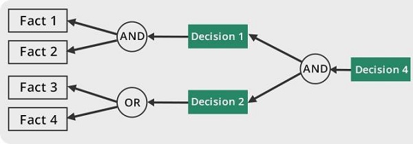
Properties of Backward-Chaining

The following outlines the key properties of backward chaining, a reasoning method that starts with a goal and works backward to find supporting facts −

• The process of reasoning begins with a conclusion that needs to be supported. Rather than progressing from facts to conclusions, it works in the opposite direction, starting with the conclusion and looking for evidence to back it up.

• It focuses solely on the necessary facts to achieve the desired conclusion or decision.

• Each rule is analyzed to determine whether it leads to the desired outcome, with facts verified throughout the process.

• The reasoning process is considered successful when the system identifies facts that support its decision.

• This approach is often used in medical diagnosis, where an algorithm works backward to determine potential diseases based on observed symptoms.

• Instead of sifting through all available data, it focuses on the most relevant information, which can lead to faster results in certain situations.

• For this method to be effective, a clear hypothesis or question must be established. If there are no facts that meet the necessary criteria, the algorithm will be unable to reach a conclusion.

• This technique is utilized in AI systems that require justification for their decisions, such as legal expert systems and fraud detection.

Example 1

Business Example: A manufacturing company encounters an unexpected increase in product issues. It starts by questioning why there are more problems and then traces back to explore potential causes, including equipment malfunctions, the quality of raw materials, and errors made by personnel.

Example 2

Healthcare Example: In medicine, a doctor tries to figure out if a patient has pneumonia. Rather than checking every possible condition, the diagnostic system begins with the end goal (pneumonia) and looks at specific symptoms like fever, chest pain, and trouble breathing before reaching a conclusion.

Example 3

Crime Investigation Example: The police start a robbery investigation by trying to identify the suspect. They work backwards by looking at evidence watching security footage, and choosing suspects based on motive and past criminal records.

Limitations of Backward Chaining

Backward chaining begins with a specific objective and works backward to gather supporting information however, it has few drawbacks −

• Dependence on Goal Selection: It requires a well-defined goal; choosing the wrong goal can result in faulty reasoning.

• Complexity: When numerous rules can support a goal, it may be difficult to identify the best option.

• Inefficiency: If the goal has many dependencies, it may require extensive backtracking, making the process slow.

Forward Chaining

Forward chaining is a data-driven inference method that begins with established facts and applies rules to derive new information until a specific goal is reached. This approach is widely used in expert systems, recommendation engines, and automated decision-making processes.

Example

A fire alarm system is designed to detect both smoke and heat. The principle "If smoke and heat are detected, sound the alarm" is activated when both conditions are met, prompting the system to sound the alarm.

Backward Chaining

Backward chaining, on the other hand, is a goal-oriented reasoning technique that starts with a hypothesis and works backward to verify supporting evidence. It is commonly utilized in AI-driven diagnostic systems, legal reasoning, and troubleshooting applications.

Example

When a doctor is diagnosing a fever, they may begin with the statement, "The patient has the flu." To verify this diagnosis, the doctor looks for additional symptoms like fever, body aches, and fatigue.

Differences between Forward Chaining and Backward Chaining

The following table highlights the major differences between Forward Chaining and Backward Chaining −

Forward Chaining	Backward Chaining
Forward Chaining starts from known facts and applies rules to derive new facts until the goal is reached.	Backward Chaining starts from the goal and works backward to find supporting facts.
Starts with known facts and observations.	Starts with a hypothesis or goal.
Searches through large amount of unnecessary data.	Searches only relevant parts of the knowledge base.
Moves from facts to conclusions (goal).	Moves from goals to facts
Data-Driven Reasoning − Processes all possible facts until a goal (or multiple goals) is reached.	Goal-Driven Reasoning − Checks only relevant rules needed to prove the goal.
Can be inefficient if the number of rules is large because it may derive unnecessary facts.	More efficient if the goal is known in advance, as it only searches relevant rules.
Used when exploring all possible outcomes from given facts.	Used when there is a specific goal to prove.
More complex due to the need to process all facts.	Less complex when there are fewer goals.
An approach known as "breadth-first search" is used in forward chaining reasoning.	A depth-first search methodology is used in backward chaining reasoning.
For example, an AI assistant processing a user's query and applying all related knowledge to provide multiple suggestions.	For example, a doctor starts by suspecting a disease (goal) and asks about symptoms to confirm it.
Best suited for applications where new knowledge must be discovered (e.g., recommendation systems).	Best suited for applications where a decision needs justification (e.g., expert systems).

Utility Theory in Artificial Intelligence

Utility Theory is an important concept in Artificial Intelligence used for rational decision-making. It provides a mathematical framework that allows intelligent agents to evaluate different states, actions, and outcomes based on numerical values called utilities. These utilities represent the level of desirability, satisfaction, or preference the agent has for a particular state.

Meaning of Utility

Utility is a numerical score assigned to each possible state or outcome.
Higher utility = more preferred outcome.

For example:

• Utility(Winning) = 100

• Utility(Drawing) = 50

• Utility(Losing) = 0

This helps the agent decide which state is best.

What is Utility Theory?

Utility Theory defines how an intelligent agent:

1. Assigns utilities to states

2. Compares outcomes based on preference

3. Chooses actions that maximize the utility or expected utility

A rational agent behaves in a way that maximizes its utility value.

Utility Function

A utility function U(s) maps each environment state s to a real number.
It allows the agent to measure how desirable each state is.

Example:

• U(Sunny Day) = 80

• U(Rainy Day) = 10

Thus, the agent prefers “Sunny Day.”

Expected Utility

When outcomes are uncertain, the utility of an action must consider probabilities.

Formula:
Expected Utility = Σ [Probability(outcome i) × Utility(outcome i)]

This is used when actions have multiple possible results.

Principle of Maximum Expected Utility (MEU)

A rational agent always chooses:
Action = arg max ExpectedUtility(action)

This principle is central to decision theory, planning, and reinforcement learning.

Types of Utility

1. Ordinal Utility – ranks preferences
   Example: A > B > C

2. Cardinal Utility – gives exact numerical values
   Example: U(A)=100, U(B)=60

Example: Utility-Based Decision Making

An intelligent agent must decide whether to drive fast or slow.

Given:

Fast Driving:

• Probability(safe) = 0.90, Utility(safe)=90

• Probability(accident)=0.10, Utility(accident)= -500

Slow Driving:

• Probability(safe)=0.99, Utility(safe)=80

• Probability(accident)=0.01, Utility(accident)= -200

Expected Utility Calculation

1. Fast Drive
= (0.90 × 90) + (0.10 × -500)
= 81 – 50
= 31

2. Slow Drive
= (0.99 × 80) + (0.01 × -200)
= 79.2 – 2
= 77.2

Decision

Since 77.2 > 31, the agent chooses Slow Drive.
Thus, the agent behaves rationally by maximizing expected utility.

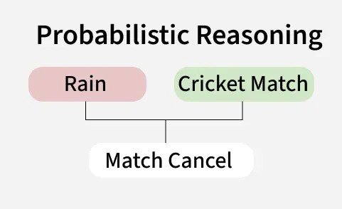
Probabilistic reasoning in Artificial Intelligence (AI) is a method that uses probability theory to manage and model uncertainty in decision-making. Unlike traditional systems that depend on precise information, it understands that real-world data is often incomplete, unclear or noisy. By giving probabilities to different possibilities, AI systems can make better decisions, predict outcomes and solve problems even when things are uncertain. This approach is important for building smart systems that can work in changing environments and make good choices in complex situations.

Probabilistic Reasoning

Need for Probabilistic Reasoning in AI

Probabilistic reasoning with artificial intelligence is important to different tasks such as:

• Machine Learning: It helps algorithms learn from incomplete or noisy data, refining predictions over time.
• Robotics: It enables robots to navigate and interact with dynamic and unpredictable environments.
• Natural Language Processing: It helps AI understand human language which is often ambiguous and depends on context.
• Decision Making: It allows AI systems to evaluate different outcomes and make better decisions by considering the likelihood of various possibilities.

Key Concepts in Probabilistic Reasoning

Probabilistic reasoning helps AI systems make decisions and predictions when they have to deal with uncertainty. It uses different ideas and models to understand how likely things are even when we don't have all the answers. Let's see some of the important concepts:

1. Probability: It is a way to measure how likely something is to happen, typically expressed as a number between 0 and 1. In AI, we use probabilities to understand and make predictions when the information we have is uncertain or incomplete.

2. Bayes' Theorem: It helps AI systems update their beliefs when they get new information. It’s like changing our mind about something based on new evidence. This is useful when we need to adjust our predictions after learning new facts.

$P(A\mid B)=\frac{P(B\mid A)\cdot P(A)}{P(B)}$

Where:

• $P(A\mid B)$: Probability of A happening, given B has happened (posterior probability).
• $P(B\mid A)$: Probability of B happening, given A happened.
• $P(A)$: Prior probability of A.
• $P(B)$: Probability of observing B.

3. Conditional Probability: It is the chance of an event happening, given that something else has already happened. This helps when the outcome depends on something that happened before.

4. Random Variables: They are values that can change or vary based on uncertainty. In simple terms, these are the things AI tries to predict or estimate. The possible outcomes of these variables depend on probability.

Types of Probabilistic Models

There are different models that use these concepts to help AI systems make sense of uncertainty. Let’s see some of them:

1. Bayesian Networks: They are graphs that show how different variables are connected with probabilities. Each node represents a variable and the edges show how they depend on each other. These networks help us understand how one piece of information can affect another.
2. Markov Models: They predict the future state of a system based only on the present state with no regard for the past. This is known as the "memoryless" property which means the future depends only on the current situation not the history that led to it.
3. Hidden Markov Models (HMMs): They extend Markov models by introducing hidden states that cannot be directly observed. These models help infer the hidden states based on observable data, using statistical techniques to estimate the likelihood of these unobservable conditions.
4. Probabilistic Graphical Models: It combine the features of Bayesian networks and Hidden Markov Models, allowing more complex relationships between variables to be represented. It provide a framework for managing uncertainty in large systems where many variables are connected and interact with each other.
5. Markov Decision Processes (MDPs): They are used for decision-making, particularly in reinforcement learning. It model an agent’s interaction with an environment where the agent takes actions that affect the state of the environment and receives rewards or penalties based on those actions.

Techniques in Probabilistic Reasoning

1. Inference: It calculates the probability of an outcome based on known data. Exact methods like variable elimination and approximate methods like Markov Chain Monte Carlo (MCMC) are used, depending on the complexity of the system.
2. Learning: It updates the parameters of probabilistic models as new data comes in, improving predictions. Techniques like maximum likelihood estimation and Bayesian estimation allow models to adapt and become more accurate over time.
3. Decision Making: AI uses probabilistic reasoning to make decisions that maximize expected rewards. Partially Observable Markov Decision Processes (POMDPs) are used when some information is hidden.

How Probabilistic Reasoning Enhances AI Systems?

Probabilistic reasoning helps AI systems navigate uncertainty, enabling them to make better decisions even when information is unclear. Let's see how it works:

1. Quantifying Uncertainty: Probabilistic reasoning turns uncertainty into probabilities. Instead of a simple “yes” or “no,” it provides a probability, like “there’s a 60% chance of rain tomorrow.”
2. Reasoning with Evidence: As new information comes in, AI systems update their predictions. For example, if dark clouds appear, the chance of rain might rise to 80%. This continuous adjustment helps AI stay accurate.
3. Learning from Past Experiences: AI systems can improve predictions by learning from historical data. For example, weather predictions become more accurate as the AI system accounts for past seasonal trends.
4. Effective Decision-Making: It allows AI to make informed decisions by considering the likelihood of different outcomes. It helps AI weigh possible paths and choose the best option even when the future is uncertain.

Applications of Probabilistic Reasoning in AI

Probabilistic reasoning is applicable in a variety of domains which includes:

1. Robotics: In robotics, probabilistic reasoning helps with navigation and mapping. For example, in Simultaneous Localization and Mapping, robots create maps and track their position in unknown environments.
2. Healthcare: AI systems use probabilistic models to predict disease likelihood and assist in diagnosis. Bayesian networks can model medical factors like symptoms and test results to guide decisions.
3. Natural Language Processing: In tasks like speech recognition and translation, models like Hidden Markov Models (HMMs) help AI understand and process ambiguous language.
4. Finance: Probabilistic reasoning in finance helps predict market trends and assess risks. Techniques like Bayesian inference and Monte Carlo simulations model financial uncertainties for better decision-making.

Advantages of Probabilistic Reasoning

• Flexibility: Probabilistic models can handle different kinds of uncertainty and can be adapted to work in various fields from healthcare to robotics.
• Robustness: These models remain effective even when the data is noisy or incomplete, making them reliable in real-world scenarios where perfect data is rarely available.
• Transparency: It provides a clear framework for understanding and explaining uncertainty which helps build trust and improve the interpretability of AI decisions.
• Scalability: It can scale to handle large amounts of data and complex systems, making them suitable for applications like big data analysis and large-scale decision-making processes.
• Decision Support: These models assist in making informed decisions under uncertainty by calculating the likelihood of different outcomes, helping AI systems choose the best course of action based on expected results.

Challenges of Probabilistic Reasoning

Despite its various advantages, probabilistic reasoning in AI also has several challenges:

1. Complexity: Some models such as large Bayesian networks can become computationally expensive, especially as the number of variables grows. This can slow down processing and limit scalability.
2. Data Quality: Probabilistic models heavily rely on accurate and clean data. If the data is noisy, incomplete or biased, the model’s predictions can become unreliable, leading to incorrect conclusions.
3. Interpretability: Understanding how probabilistic models make decisions can be tough, particularly in complex systems or deep learning models. This makes it harder to trust and explain AI decisions to non-experts.

Hidden Markov Models

Introduction

A Hidden Markov Model (HMM) is a statistical model used in Artificial Intelligence to represent systems that are probabilistic and have hidden (unobserved) states.
In many real-life problems, we cannot directly observe the internal state of the system, but we can observe some output. HMM helps us understand these hidden states using the observed data.

Uses of Hidden Markov Models

HMMs are widely used in AI because they handle time-series, uncertainty, and sequential data. Some important uses are:

1. Speech Recognition
   The spoken sound is observed, but the correct word or phoneme (hidden state) must be predicted.

2. Natural Language Processing
   Used in POS tagging, sentence prediction, text classification, etc.

3. Bioinformatics
   Used to predict gene sequences and protein structures.

4. Activity Recognition
   Predicting human activity from sensor data (walking, running, sitting).

5. Weather Prediction
   Weather condition (hidden) predicted from observable events.

6. Machine Translation
   Used for probabilistic word alignment.

Main Components of HMM

1. Hidden States – not directly seen (e.g., weather: sunny, rainy).

2. Observations – output we can see (e.g., walk, shop).

3. Transition Probabilities – probability of moving from one hidden state to another.

4. Emission Probabilities – probability of observing an output from a hidden state.

5. Initial Probabilities – probability of starting in a particular hidden state.

Example: Weather Prediction Using HMM

Assume the hidden states are:

• S1 = Sunny

• S2 = Rainy

Observations are:

• O1 = Walk

• O2 = Shop

Initial Probabilities

P(Sunny) = 0.6
P(Rainy) = 0.4

Transition Probabilities

Sunny → Sunny = 0.7
Sunny → Rainy = 0.3
Rainy → Sunny = 0.4
Rainy → Rainy = 0.6

Emission Probabilities

From Sunny:
Walk = 0.8, Shop = 0.2

From Rainy:
Walk = 0.3, Shop = 0.7

Problem:

Find the probability of observing the sequence:
Walk → Shop

Step 1: Initialization

Alpha1(Sunny) = 0.6 * 0.8 = 0.48
Alpha1(Rainy) = 0.4 * 0.3 = 0.12

Step 2: For second observation (Shop)

Sunny:
(0.48 * 0.7 + 0.12 * 0.4) * 0.2
= (0.336 + 0.048) * 0.2
= 0.384 * 0.2
= 0.0768

Rainy:
(0.48 * 0.3 + 0.12 * 0.6) * 0.7
= (0.144 + 0.072) * 0.7
= 0.216 * 0.7
= 0.1512

Total Probability

P(Walk, Shop) = 0.0768 + 0.1512
= 0.228

Bayesian Belief Network

Bayesian belief network is key computer technology for dealing with probabilistic events and to solve a problem which has uncertainty. We can define a Bayesian network as:

"A Bayesian network is a probabilistic graphical model which represents a set of variables and their conditional dependencies using a directed acyclic graph."

It is also called a Bayes network, belief network, decision network, or Bayesian model.

Bayesian networks are probabilistic, because these networks are built from a probability distribution, and also use probability theory for prediction and anomaly detection.

Real world applications are probabilistic in nature, and to represent the relationship between multiple events, we need a Bayesian network. It can also be used in various tasks including prediction, anomaly detection, diagnostics, automated insight, reasoning, time series prediction, and decision making under uncertainty.

Bayesian Network can be used for building models from data and experts opinions, and it consists of two parts:

• Directed Acyclic Graph
• Table of conditional probabilities.

The generalized form of Bayesian network that represents and solve decision problems under uncertain knowledge is known as an Influence diagram.

A Bayesian network graph is made up of nodes and Arcs (directed links), where:

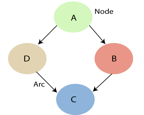
• Each node corresponds to the random variables, and a variable can be continuous or discrete.
• Arc or directed arrows represent the causal relationship or conditional probabilities between random variables. These directed links or arrows connect the pair of nodes in the graph.
  These links represent that one node directly influence the other node, and if there is no directed link that means that nodes are independent with each other
  • In the above diagram, A, B, C, and D are random variables represented by the nodes of the network graph.
  • If we are considering node B, which is connected with node A by a directed arrow, then node A is called the parent of Node B.
  • Node C is independent of node A.

Note: The Bayesian network graph does not contain any cyclic graph. Hence, it is known as a directed acyclic graph or DAG.

The Bayesian network has mainly two components:

• Causal Component
• Actual numbers

Each node in the Bayesian network has condition probability distribution P(X_i |Parent(X_i) ), which determines the effect of the parent on that node.

Bayesian network is based on Joint probability distribution and conditional probability. So let's first understand the joint probability distribution:

Joint probability distribution:

If we have variables x1, x2, x3,....., xn, then the probabilities of a different combination of x1, x2, x3.. xn, are known as Joint probability distribution.

P[x₁, x₂, x₃,....., x_n], it can be written as the following way in terms of the joint probability distribution.

= P[x₁| x₂, x₃,....., x_n]P[x₂, x₃,....., x_n]

= P[x₁| x₂, x₃,....., x_n]P[x₂|x₃,....., x_n]....P[x_n-1|x_n]P[x_n].

In general for each variable Xi, we can write the equation as:

P(Xi|Xi-1,........., X1) = P(Xi |Parents(Xi ))

Explanation of Bayesian network:

Let's understand the Bayesian network through an example by creating a directed acyclic graph:

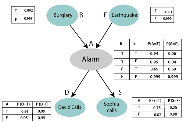
Example: Harry installed a new burglar alarm at his home to detect burglary. The alarm reliably responds at detecting a burglary but also responds for minor earthquakes. Harry has two neighbors David and Sophia, who have taken a responsibility to inform Harry at work when they hear the alarm. David always calls Harry when he hears the alarm, but sometimes he got confused with the phone ringing and calls at that time too. On the other hand, Sophia likes to listen to high music, so sometimes she misses to hear the alarm. Here we would like to compute the probability of Burglary Alarm.

Problem:

Calculate the probability that alarm has sounded, but there is neither a burglary, nor an earthquake occurred, and David and Sophia both called the Harry.

Solution:

• The Bayesian network for the above problem is given below. The network structure is showing that burglary and earthquake is the parent node of the alarm and directly affecting the probability of alarm's going off, but David and Sophia's calls depend on alarm probability.
• The network is representing that our assumptions do not directly perceive the burglary and also do not notice the minor earthquake, and they also not confer before calling.
• The conditional distributions for each node are given as conditional probabilities table or CPT.
• Each row in the CPT must be sum to 1 because all the entries in the table represent an exhaustive set of cases for the variable.
• In CPT, a boolean variable with k boolean parents contains 2^K probabilities. Hence, if there are two parents, then CPT will contain 4 probability values

List of all events occurring in this network:

• Burglary (B)
• Earthquake(E)
• Alarm(A)
• David Calls(D)
• Sophia calls(S)

We can write the events of problem statement in the form of probability: P[D, S, A, B, E], can rewrite the above probability statement using joint probability distribution:

P[D, S, A, B, E]= P[D | S, A, B, E]. P[S, A, B, E]

=P[D | S, A, B, E]. P[S | A, B, E]. P[A, B, E]

= P [D| A]. P [ S| A, B, E]. P[ A, B, E]

= P[D | A]. P[ S | A]. P[A| B, E]. P[B, E]

= P[D | A ]. P[S | A]. P[A| B, E]. P[B |E]. P[E]

Let's take the observed probability for the Burglary and earthquake component:

P(B= True) = 0.002, which is the probability of burglary.

P(B= False)= 0.998, which is the probability of no burglary.

P(E= True)= 0.001, which is the probability of a minor earthquake

P(E= False)= 0.999, Which is the probability that an earthquake not occurred.

We can provide the conditional probabilities as per the below tables:

Conditional probability table for Alarm A:

The Conditional probability of Alarm A depends on Burglar and earthquake:

B	E	P(A= True)	P(A= False)
True	True	0.94	0.06
True	False	0.95	0.04
False	True	0.31	0.69
False	False	0.001	0.999

Conditional probability table for David Calls:

The Conditional probability of David that he will call depends on the probability of Alarm.

A	P(D= True)	P(D= False)
True	0.91	0.09
False	0.05	0.95

Conditional probability table for Sophia Calls:

The Conditional probability of Sophia that she calls is depending on its Parent Node "Alarm."

A	P(S= True)	P(S= False)
True	0.75	0.25
False	0.02	0.98

From the formula of joint distribution, we can write the problem statement in the form of probability distribution:

P(S, D, A, ¬B, ¬E) = P (S|A) *P (D|A)*P (A|¬B ^ ¬E) *P (¬B) *P (¬E).

= 0.75* 0.91* 0.001* 0.998*0.999

= 0.00068045.

Hence, a Bayesian network can answer any query about the domain by using Joint distribution.

The semantics of Bayesian Network:

There are two ways to understand the semantics of the Bayesian network, which is given below:

1. To understand the network as the representation of the Joint probability distribution.

It is helpful to understand how to construct the network.

2. To understand the network as an encoding of a collection of conditional independence statements.

It is helpful in designing inference procedure.

Ques.  Write a short note on Bayesian network.

 Or 

Explain the Bayesian network by taking an example . How is the Bayesian network representation for uncertainty knowledge ?

Answer:

• A Bayesian network is a probabilistic graphical model(PGM) which represents a set of variables and their conditional dependencies using a directed acyclic graph(DAG).
• These networks are built from a probability distribution, and also use probability theory for prediction and anomaly detection.
• Each  variable  is  associated  with  a  conditional  probability  table  which  gives  the probability  of  this  variable  for  different  values  of  the  variables  on  which  this  node depends.
• Using this model, it is possible to perform inference and learning.Bayesian  networks  that  model  a  sequence  of  variables  varying  in  time  are  called dynamic Bayesian networks
• Bayesian   networks   with   decision   nodes   which   solve  decision   problems   under uncertainly are Influence diagrams.

Explicit representation of conditional independencies Missing arcs encode conditional independence Efficient representation of joint PDF P(X) Generative model (not just discriminative): allows arbitrary queries to be answered, 

e.g. P (lung cancer=yes | smoking=no, positive X-ray=yes ) = ?

For example, a Bayesian network could represent the probabilistic relationships between diseases and symptoms. Given symptoms, the network can be used to compute the probabilities of the presence of various diseases. Efficient algorithms can perform inference and learning in Bayesian networks.

Another Example:

Applications:

• Prediction
• Anomaly detection
• Diagnostics
• Automated insight
• Reasoning
• Time series prediction
• Decision making under uncertainty.

 

 

Ques. Explain the role of  prior probability and posterior probability in bayesian classification. 

Answer:

Prior Probability:

Bayesian statistical inference is the probability of an event before new data is collected.This is the best rational assessment of the probability of an outcome based on current knowledge.

It shows the likelihood of an outcome in a given dataset.

For example,

In the Mortgage case, P(Y) is the default rate on a home mortgage, which is 2%. P(Y|X) is called the conditional probability, which provides the probability of an outcome given the evidence, that is, when the value of X is known.

Posterior Probability:

It is calculated using Bayes’ Theorem.Prior probability gets updated when new data is available,to produce a more accurate measure of a potential outcome.

A posterior probability can subsequently become a prior for a new updated posterior probability as new information arises and is incorporated into the analysis.

Ques. Explain the method of handling approximate inference in Bayesian networks.

Answer:

Inference over a Bayesian network can come in two forms. The first is simply evaluating the joint probability of a particular assignment of values for each variable (or a subset) in the network

In exact inference, we analytically compute the conditional probability distribution over the variables of interest.

Methods of handling approximate inference in Bayesian Networks:

Simulation Methods:

It uses the network to generate samples from the conditional probability distribution and estimate conditional probabilities of interest when the number of samples is sufficiently large.

With machine learning, the inputs are known exactly, but the model is unknown prior to training. Regarding output, the differences are more subtle. Both give an output, but the source of uncertainty is different.

Variational Methods:

Variational Bayesian methods are a family of techniques for approximating intractable integrals arising in Bayesian inference and machine learning.